All published articles of this journal are available on ScienceDirect.

Corrosion of Mild Steel and Galvanized Steel in SO2 Enclosures: The Incidence of Negative Gravimetric Corrosion Rates
Authors Info & Affiliations
Abstract
Background
Corrosion rates are frequently calculated from the weight loss of material samples, and they provide a measure of the degree of material degradation that has occurred when exposed to corrosive environments. However, some metal samples that have been exposed to corrosive environments experience negative weight loss, or more accurately, positive weight gain, which results in a negative corrosion rate. In the corpus of research on corrosion studies, there is little evidence for the occurrence of negative gravimetric corrosion rate in metals.
Methods
In this work, we employed gravimetric analysis to study the atmospheric corrosion of mild steel and galvanized steel in Sulphur (IV) oxide (SO2) enclosures or chambers for a period of 2 weeks and 4 weeks. The results indicated weight gain of the metals after exposure to the SO2-polluted atmospheric environment in the enclosures, thereby leading to negative corrosion rates. In seeking more insight to explain the observed phenomenon, XRF (X-Ray Fluorescence), SEM (Scanning electron microscopy) and FTIR (Fourier Transform Infrared Spectroscopy) analyses were conducted on the metal coupons.
Results
While the XRF results show a consistent reduction in the iron (Fe) content of the samples with a lesser percent iron composition observed with increasing exposure time, the SEM results reveal the formation of crystalline corrosion products on the metal surfaces. The FTIR results also indicated the pronounced presence of hydroxyl functional groups.
Conclusion
Both the XRF and SEM results indicate that the active components of the metal samples are being used up in the surface electrochemical reactions and are converted to visible corrosion products which are responsible for the weight gain. Concluding from the FTIR results, the presence of corrosion products Fe(OH)2 and Fe(OH)3 is confirmed among others.
1. INTRODUCTION
Air pollution, emanating from anthropogenic sources via industrial and vehicular activities, has become a major environmental issue of global concern due to the harmful effects it has on health, safety and the environment [1, 2]. Naturally, nearly all metals corrode when exposed to the atmosphere due to the presence of corrosive pollutants in the air [3, 4]. These pollutants include gases like Sulphur (IV) oxide (SO2) which can degrade or deteriorate the surfaces of metals like mild steel and galvanized steel. As such, corrosion studies which further elucidate the effect of this corrosive gas are needed. Others that explore inhibitive strategies of SO2 corrosion are also being progressed [5, 6].
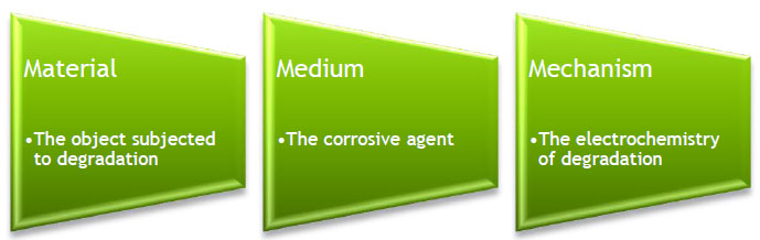
Corrosion is the outcome of the interaction of three key essential requirements (which can be termed the 3 M’s of corrosion): the material, the medium and the mechanism, as depicted in Fig. (1). Corrosion becomes evident when the electrochemical reaction (the mechanism) takes its effect on the object (the material) under the influence of the corrosive environment (the medium). Although all materials undergo some form of degradation over time, however, of all materials, metals are the most susceptible to corrosion or degradation. Almost always, when gravimetric analysis is used to monitor the process, corrosion results in the weight loss of the metallic material indicating the loss of some of the active material which had been degraded by the electrochemical reaction occurring on its surface due to the impact of the exposure to the corrosive environment. Metallic corrosion occurs often in steel materials like mild steel and galvanized steel and is visibly observable in steel structures and equipment by the formation of rust [7]; it can also be noticeable by weight loss.
Corrosion rates are often computed from the weight loss of the material samples and they give the indication of the level of degradation the material has undergone when exposed to the corrosive environment [8-11]. High corrosion rates are indicative of the higher level of degradation while lower corrosion rates depict lesser material degradation. Corrosion rates are often reported as positive values computed from Eq. (1) [12]:
 |
(1) |
where rcorr is the corrosion rate [g/(m2 h)], ∆m is the weight loss (g), A is the surface area (m2), and t is the exposure time (h).
However, negative weight loss, or more aptly, weight gain, by metal samples after exposure to a corrosive environment results in a negative corrosion rate. The phenomenon of negative gravimetric corrosion rate in metals is scarcely observed and has limited evidence in the body of literature on corrosion studies. The occurrence of the phenomenon has been attributed to a number of reasons, often peculiar and unique to the study in which it is observed.
Chen et al. (2014) [13] reported the incidence in their study aimed to better understand how sulphur (IV) oxide (SO2) affects the corrosion of low alloy steel in artificial coastal industrial environments. The findings show that the steel's corrosion weight gain first rises with an increase in SO2 content up to a certain point and subsequently falls with an increase in SO2 content. In the work, the authors noted that the observed weight gain was due to the synthesis of γ-FeOOH at the initial increase in SO2 and the inhibition of the same (with the formation of α-FeOOH) at higher SO2 levels. In another work, Lee et al. (2017) [14] also observed weight gain in their study of the corrosion of carbon steel under three different gaseous atmospheres. Their results show weight gains of the carbon steel after corrosion in air, Ar/1%SO2-, and Ar/0.1%H2S-mixed gas. They observed that the weight gains increased swiftly with an increase in temperature.
In this present research, the corrosion of mild steel and galvanized steel samples exposed to SO2 environment in enclosed chambers was studied. In addition to aiding in the understanding of how SO2 in a polluted enclosed environment affects the corrosion of mild steel and galvanized steel, this research seeks to study the observed phenomenon of weight gain resulting from atmospheric corrosion.
2. MATERIALS AND METHODS
2.1. Preparation of Metal Samples
Samples of the metals (mild steel and galvanised steel) were procured from an engineering research institute in Nigeria and prepared into coupons of dimensions 30mm × 20mm × 2mm. The metal coupons were polished by polishing papers and then rinsed in deionized water before being degreased in acetone.
2.2. Creating Simulated SO2-polluted Air
Atmospheric conditions polluted with sulphur (IV) oxide (SO2) were simulated by creating a chamber made of an air-tight box where a prepared solution of SO2 is stored. The solution gives off SO2 gas in the chamber thereby creating a SO2-polluted atmosphere in the chamber which can be used for the atmospheric corrosion tests to be carried out. The recommended boxes were transparent plastic boxes with tightly fitting lids with typical dimensions 18 x 10 x 8 cm [15].
The SO2 solution was prepared from sodium metabisulfite (Na2S2O5) and sulphuric acid (H2SO4) following the procedure outlined by the Royal Society of Chemistry (2022) [15] not more than 24 hours in advance of the intended usage. In a fume cupboard, 9.5 g of sodium metabisulfite was dissolved in 100 cm3 of water. Then, 100 cm3 of 0.5 M H2SO4 was added and then made up to 250 cm3 with water. The solution was then stored in a well-stoppered bottle and kept in a fume cupboard.
2.3. Atmospheric Corrosion Test (Exposure to Laboratory Corrosion Chamber)
About 50 cm3 of the prepared SO2 solution was poured into a beaker and placed inside one of the chambers or boxes. The beaker was first placed inside the fume cupboard before pouring the solution into it. One coupon of mild steel was placed in the box. Another coupon of galvanised steel was placed in another box following the same procedure. The boxes (with the coupons and the beakers containing the SO2 solution) were then securely covered with the lid and appropriately labelled and monitored for corrosion exposure for 14 days (2 weeks). The box would only be opened after 2 weeks. A similar procedure was followed for another set of two boxes containing the same contents (mild steel and galvanized steel coupons and 50 cm3 of SO2 solution) observed for 4 weeks (28 days) each. Each box contained a sheet of expanded polystyrene cut to fit inside the base of the box. This is to provide support to the metal samples placed on the sheet.
2.4. Surface Morphological Structure, X-Ray Fluorescence and Fourier Transform Infrared Spectroscopy Analyses of Samples
Samples of each of the two metals were scanned before the atmospheric corrosion test to obtain an image of the surface structure of the pre-exposed metals. Scanning electron microscopy (SEM) was used to achieve the surface analysis. At the end of the atmospheric corrosion tests, the metal samples were subjected to SEM for analysis of the surface structures of the exposed metals.
The samples were also analysed by X-Ray Fluorescence (XRF) to reveal the elemental compositions of the exposed/corroded coupons and the unexposed control samples. Furthermore, Fourier Transform Infrared Spectroscopy (FTIR) analysis was also carried out on the samples.
2.5. Determination of Corrosion Rates of Samples
The mild steel and galvanized steel coupons were weighed before being placed in the SO2 enclosures and after 2 and 4 weeks of exposure to SO2 in the enclosures.
The corrosion rates of the exposed samples were determined by gravimetric analysis using the following equation [12]:
|
where rcorr is the corrosion rate [g/(m2 h)], ∆m is the weight loss (g), A is the surface area (m2), and t is the exposure time (h).
3. RESULTS AND DISCUSSION
3.1. Gravimetric Analysis and Corrosion Rate Results
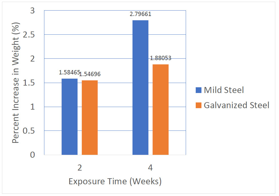
After exposure to the SO2 enclosures containing 50cm3 of SO2 solution prepared from sodium metabisulfite and sulphuric acid, the weights of the mild steel and galvanized steel coupons were measured and compared with the weights of the same samples before the exposure to the corrosive environment. A weight gain was observed for all four samples as summarized in Table 1. The observed weight gain increased with a longer exposure period. For mild steel, a weight gain of 0.33g was observed after 4 weeks compared to a lesser weight gain of 0.19g for an exposure time of 2 weeks. A similar trend was observed for galvanized steel as well with an increased weight gain of 0.17g for a 4-week exposure period in comparison to a lesser weight gain of 0.14g after 2 weeks of exposure. To give a better insight into the observed increase in weight of the samples, the percent increase in weight was computed and displayed in Fig. (2). Mild steel experienced a greater percent increase in weight than galvanized steel for both periods of exposure. In comparison to galvanized steel, the percent increase in weight was more pronounced in the 4-week exposure period in mild steel with a weight gain of nearly 2.8% in contrast to the 1.88% weight increase in the former.
| Sample # | Material |
Exposure Time (Weeks) |
Weight Gain (g) |
Corrosion Rate (g/m2-h) |
|---|---|---|---|---|
| MS-1 | Mild Steel | 2 | 0.19 | -0.41579 |
| MS-2 | Mild Steel | 4 | 0.33 | -0.36108 |
| GS-3 | Galvanized Steel | 2 | 0.14 | -0.30637 |
| GS-4 | Galvanized Steel | 4 | 0.17 | -0.18601 |
The corresponding corrosion rates were calculated using equation (1) and the results are also displayed in Table 1. The corrosion rates obtained are negative with higher values (less negative) observed for the 4-week period of exposure for both mild steel and galvanized steel, and lower values (more negative) observed for the 2-week exposure time. This implies that the extent of corrosion or degradation was more when the metal samples were exposed for longer periods indicating an increase in corrosion with time.
The interpretation of the concept of corrosion rate itself is similar to the general concept of the rate of reaction. The rate of any reaction can be interpreted in terms of the reactants and the products. Defined in terms of a reacting species, the rate of reaction is the rate of disappearance of a reactant; and the rate of appearance or formation of a product (when defined in terms of the product). Hence for a reacting species, the instantaneous concentration of the reactant at any time during the course of the reaction or at the end of the reaction is less than its initial concentration or its concentration at the start of the reaction. This difference is always negative for the reactant (final concentration minus initial concentration) and so is the rate of change of the concentration of the reactant with respect to time. For products, the difference is always positive with the final concentration of the product being greater than its initial concentration.
The corrosion rate itself has a notion of the loss or depletion of a metallic substance (the reactant). It is like defining the rate of change of a reactant species bearing in mind that that there is going to be a definite loss of the reacting species (the metal). Hence, the definition of the corrosion rate has been defined with the numerator as weight loss, that is, the difference between the initial and the final weight of the reacting metal, giving a positive value. Ideally, this should be negative, final minus initial, going by the convention of the definition of the rate of a reaction. Hence, the generally observed positive values for corrosion rate are due to the use of the initial minus final difference. It is like saying the rate of disappearance or loss of the metal is a certain value (the actual magnitude) of the rate of loss of the metal. So, corrosion rate reports only the magnitude of the rate of weight loss (of the metal) and not the direction whether increase or decrease of the rate of reaction.
Given this background, the observation of a negative corrosion rate therefore indicates that there is an obvious increase in the weight of the sample, hinting at the presence or formation of a corrosion product in a large amount observable by the weight gain. It means the reacting surface has led to the formation of a product whose final weight is more than its initial weight. Likewise, it can also mean that the rate of disappearance or depletion of the reactant metal is so much that the formation of corrosion products has been greatly favoured and has outweighed the amount of metal left.
Since the corrosion rate is obtained from the gross weight of the metal sample and not by the weight of the actual active reacting species or the formation of products, it is difficult to tell which species (product formed) led to the weight gain or to what extent it has been formed. Also, it does not tell to what extent the active component of the reactant metal has been depleted. We only have the magnitude of the overall weight of the sample consisting of both the reactant and the product formed.
3.2. XRF Results
The XRF results showing the elemental compositions of the mild steel samples MS-1 (exposed for 2 weeks), MS-2 (exposed for 4 weeks) and the unexposed control, are presented in Table 2. When compared with the control unexposed sample, an observable decrease was recorded in the compositions of iron, copper and silicon in the two corroded samples. Iron, copper and silicon compositions are consistently reduced with increasing periods of exposure to the corrosive environment indicative of a possible degradation and conversion of the said elemental components to other corrosion products.
A similar trend was also observed for the galvanized steel coupons as shown by the XRF results reported in Table 3 for iron, carbon and silicon. Whereas in the corroded mild steel samples, copper composition reduced consistently with increasing exposure time, in galvanized steel it was not so. Only iron and silicon, as was observed for the mild steel coupons, followed the trend of reducing the weight compositions of the elements, as well as carbon. Again, the consistent decrease of the elemental iron content of the corroded samples (GS-3 and GS-4) with an exposure time of 2 and 4 weeks, respectively when compared with the unexposed control sample, could be a result of the degradation and electrochemical conversion of the element in the metal to other corrosion products which became responsible for the overall weight gain of the coupons as earlier stated.
| S/N | Element | Symbol | Composition (wt %) | |||
|---|---|---|---|---|---|---|
| Control-MS | MS-1 | MS-2 | ||||
| 1 | Carbon | C | 0.143 | 0.153 | 0.137 | |
| 2 | Silicon | Si | 0.303 | 0.259 | 0.25 | |
| 3 | Aluminum | Al | 0.004 | 0.004 | 0.003 | |
| 4 | Iron | Fe | 96.217 | 96.001 | 95.986 | |
| 5 | Zinc | Zn | 0.005 | 0.005 | 0.005 | |
| 6 | Phosphorus | P | 0.014 | 0.024 | 0.013 | |
| 7 | Sulphur | S | 0.038 | 0.041 | 0.037 | |
| 8 | Lead | Pb | 0.002 | 0.002 | 0.002 | |
| 9 | Manganese | Mn | 0.538 | 0.571 | 0.563 | |
| 10 | Chromium | Cr | 0.908 | 0.911 | 0.895 | |
| 11 | Nickel | Ni | 0.208 | 0.204 | 0.199 | |
| 12 | Molybdenum | Mo | 0.48 | 0.569 | 0.553 | |
| 13 | Arsenic | As | 0.027 | 0.026 | 0.021 | |
| 14 | Cobalt | Co | 0.025 | 0.028 | 0.024 | |
| 15 | Tin | Sn | 0.029 | 0.02 | 0.022 | |
| 16 | Copper | Cu | 0.251 | 0.198 | 0.193 | |
| 17 | Vanadium | V | 0.004 | 0.004 | 0.003 | |
Table 3.
| S/N | Element | Symbol | Composition (wt %) | |||
|---|---|---|---|---|---|---|
| Control-GS | GS-3 | GS-4 | ||||
| 1 | Carbon | C | 0.182 | 0.177 | 0.174 | |
| 2 | Silicon | Si | 0.236 | 0.235 | 0.21 | |
| 3 | Aluminum | Al | 0.501 | 0.251 | 0.393 | |
| 4 | Iron | Fe | 98.365 | 98.13 | 98.021 | |
| 5 | Zinc | Zn | 0.005 | 0.004 | 0.004 | |
| 6 | Phosphorus | P | 0.006 | 0.01 | 0.009 | |
| 7 | Sulphur | S | 0.02 | 0.026 | 0.016 | |
| 8 | Lead | Pb | 0.003 | 0.003 | 0.003 | |
| 9 | Manganese | Mn | 0.453 | 0.702 | 0.613 | |
| 10 | Chromium | Cr | 0.026 | 0.055 | 0.058 | |
| 11 | Nickel | Ni | 0.038 | 0.075 | 0.069 | |
| 12 | Molybdenum | Mo | 0.004 | 0.003 | 0.01 | |
| 13 | Arsenic | As | 0.004 | 0.004 | 0.004 | |
| 14 | Cobalt | Co | 0.006 | 0.007 | 0.007 | |
| 15 | Tin | Sn | 0.007 | 0.014 | 0.016 | |
| 16 | Copper | Cu | 0.093 | 0.209 | 0.2 | |
| 17 | Vanadium | V | 0.001 | 0.003 | 0.003 | |
3.3. Results of Scanning Electron Microscopy (SEM)
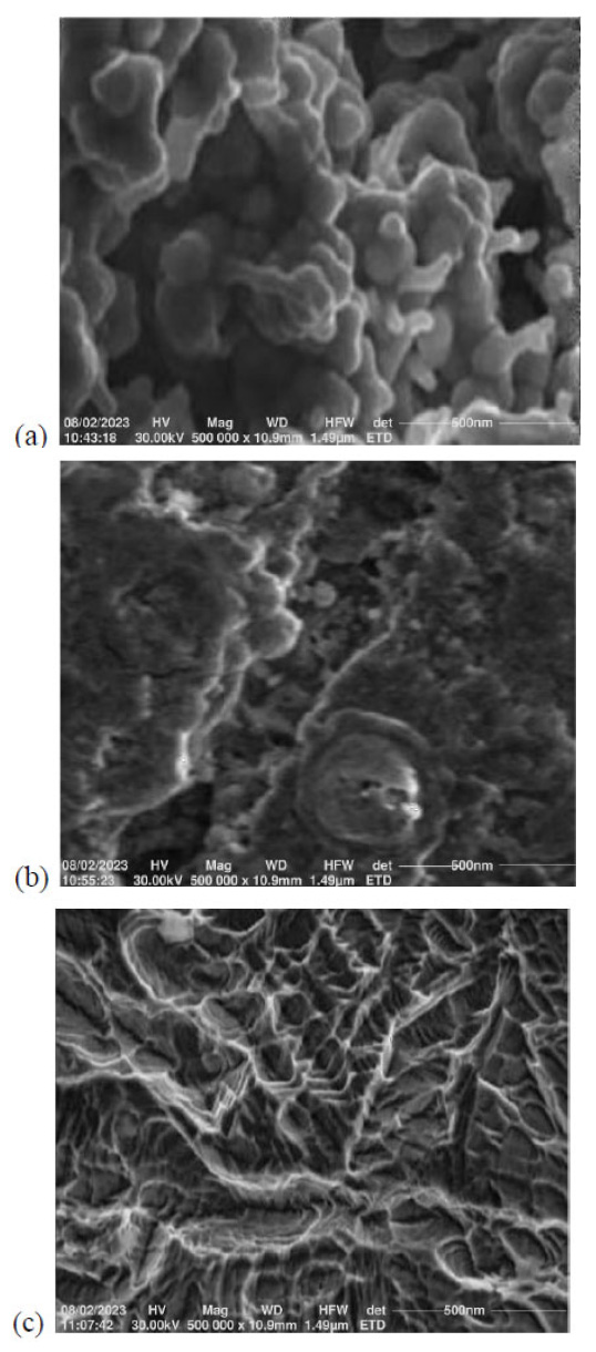
The SEM micrographs taken for the mild steel samples are shown in Fig. (3). In comparison with the control coupon, the SO2-exposed coupons have the formation of crevices and white patches which become more pronounced in the coupon with the longer time of exposure (MS-2). As expected, both the MS-1 and MS-2 coupons’ surface morphologies show the presence of films of crystalline corrosion products indicative of progressing degradation of the metals.
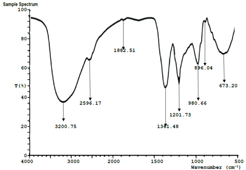
| Run # | Peak Wavelength(cm-1) | Transmittance (%) | Assignment | Functional group |
|---|---|---|---|---|
| 1 | 3200.75 | 36.10 | O-H stretching vibration. | Hydroxyl group |
| 2 | 2596.17 | 66.32 | C–H (CH2) bond stretch vibration | Alkanes |
| 3 | 1882.51 | 93.48 | C=O stretching vibration | Carboxylic acid |
| 4 | 1361.48 | 48.30 | O-H bending vibration | Hydroxyl |
| 5 | 1201.73 | 52.17 | C-H stretching vibrations | Aromatic rings |
| 6 | 980.66 | 64.52 | C–O bending vibration | Carbonyl |
| 7 | 896.04 | 92.93 | C-H stretching vibrations | Alkanes |
| 8 | 673.20 | 71.85 | C-F stretching vibrations | Fluorine group |
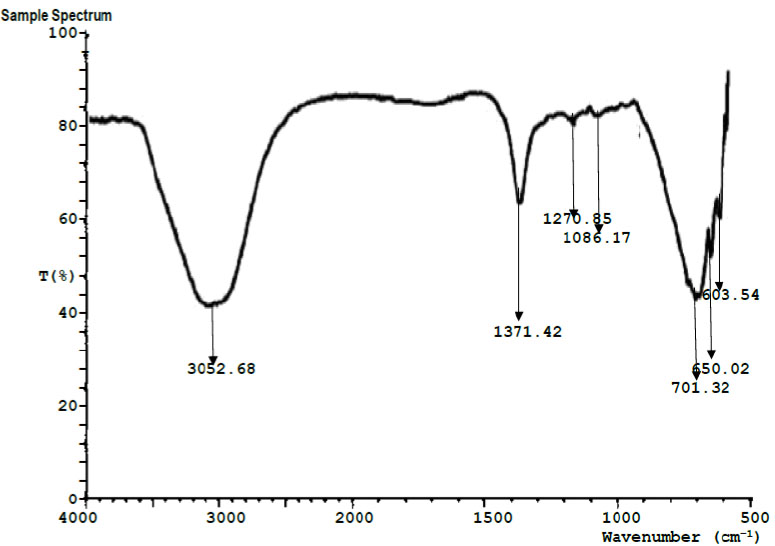
| Run # | Peak Wavelength(cm-1) | Transmittance (%) | Assignment | Functional group |
|---|---|---|---|---|
| 1 | 3058.68 | 42.75 | O-H stretching vibration | Hydroxyl group |
| 2 | 1371.42 | 65.83 | C-H stretching vibration | Alkanes |
| 3 | 1270.85 | 79.33 | –CH2 symmetric stretching vibration | alkanes |
| 4 | 1086.17 | 79.47 | -C=C- stretching vibration | Alkenes |
| 5 | 701.32 | 44.80 | C-H stretching vibrations | Aromatic rings |
| 6 | 650.02 | 52.69 | C-O stretching vibration | Carbonyl acid |
| 7 | 603.54 | 61.74 | C-F. C-Cl, C-I Stretching vibration | Alkyl halide |
3.4. Results of Fourier Transform Infrared Spectroscopy (FTIR)
Figs. (4 and 5) show the FTIR spectroscopy results for the 4-week exposed mild steel and galvanized steel, respectively. Tables 4 and 5 contain the interpretation and identification of the observed spectra peaks for the mild steel and galvanized steel, respectively. Among other functional groups, both spectra for the mild steel and galvanized steel show the high presence of hydroxyl groups (-OH). Iron hydroxide (Fe(OH)2) and iron trihydroxide (Fe(OH)3) are notable corrosion products that have been previously reported [16], whose presence may be responsible for the observed hydroxyl groups in both samples.
CONCLUSION
In this study, gravimetric analysis was employed to observe the atmospheric corrosion of mild steel and galvanized steel inside SO2 enclosures or chambers over the course of two and four weeks, respectively. The findings showed that the metals gained weight after being exposed to the SO2-polluted atmosphere in the enclosures, which caused negative corrosion rates. The metal coupons were subjected to XRF (X-Ray Fluorescence) and SEM (Scanning Electron Microscopy) investigations in an effort to get a better understanding of the event that had been seen. SEM data showed the production of crystalline corrosion products on the metal surfaces, which corroborates with the XRF results, which show a continuous decline in the iron (Fe) content of the samples with lower percent iron composition detected with increasing exposure time. The active component of the metal samples is being depleted in the surface electrochemical processes and is changed into visible corrosion products that are the cause of the weight rise, according to the XRF and SEM results. Further analysis by FTIR spectroscopy revealed the presence of key functional groups of which the hydroxyl group was prominent indicating that the corrosion products iron hydroxide (Fe(OH)2) and iron trihydroxide (Fe(OH)3) are mostly present.