All published articles of this journal are available on ScienceDirect.

A Decision-analytic Model for the Bi-objective Sizing of Heat Exchangers Under Uncertainty
Authors Info & Affiliations
Abstract
Aim
The aim of this work is to show that the preliminary sizing of process equipment, which is done relying on ranges of typical values of several key parameters, can be conveniently approached as a bi-objective “basic risky decision under uncertainty” problem from Decision Analysis.
Background
In the early stages of chemical process design, equipment sizing is done without knowing the exact value of several key process parameters. This is the case of heat exchangers, as convective heat transfer coefficients are highly sensitive to temperature, pressure, and flow conditions, which will be known with certainty only after the equipment enters operation.
Objective
This work shows how heat exchanger sizing with uncertain information can be modelled as a decision-making problem under uncertainty, from a decision-analytic point of view.
Method
The decision model consists of a factual model that produces the probability distribution of the consequences (quality of outlet temperature control and equipment cost) for the alternatives, and a value model, which provides a quantitative metric for the consequences' desirability.
Result
The results are presented as a chart showing the recommended design given the decision-maker´s relative strength of preference between equipment performance and cost.
Conclusion
Chemical process equipment design depends on physical parameters, some of which are not precisely known at the initial project stages. In said situations, equipment sizing can be stated as a decision-making problem under uncertainty and approached using Decision Analysis, as shown in this paper for the design of heat exchangers.
1. INTRODUCTION
The initial phases of chemical plant design require a preliminary economic assessment of the project. This involves an estimation of the equipment capacities and costs. The formulae for sizing process equipment require physical parameters whose value cannot be known accurately in the initial stages of the project. However, the literature offers typical ranges for the values of the required parameters, on which the engineer should rely for equipment design, applying oversizing factors to cover the uncertainties surrounding the design process [1].
On the other hand, decision analysis, being a discipline aiming to help in difficult decision making defines the structure of the “basic risky decision” as the influence diagram of Fig. (1) [2]. Decision D, shown as a rectangle, is made without knowing the value of an uncertain event I, shown as a circle. The alternative chosen and the resolution of the uncertain event fix the outcome or consequence, UG experienced by the decision maker. The hexagon UG indicates that the decision-maker has preferences for the values taken by this variable, preferring certain consequences to others. A complete model of a decision situation can be separated into a factual model, which calculates a probability distribution of the consequences given the alternatives, and a value model, which quantitatively expresses the decision-maker's preference for different consequences.
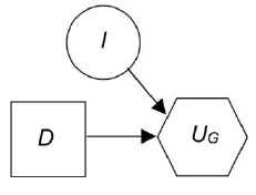
Basic risky decision.
The sizing of equipment can be put in the form of Fig. (1) if a design parameter is unknown. The decision would be the equipment size, the uncertainty would be the unknown parameter value, and the consequences the results accrued given the chosen size and true parameter value. This work treats the sizing of a heat exchanger, in uncertainty of the heat transfer parameters required for the calculations, as a basic decision under risk. One of the key uncertainties in the early design of heat exchangers is the value of the heat-transfer coefficients, as they are used to calculate the required heat transfer area, which determines the equipment performance. The ranges provided in the literature for typical values of these parameters, which can span several orders of magnitude for phase changing heat transfer processes, acknowledge this variability. It is assumed that information on the heat transfer parameters is available as ranges of possibilities, which can be found in heat exchanger design handbooks. The basic equations of heat exchange are used to develop a factual model, which provides the probability distribution of the outlet temperature given the design decisions. The value model consists of a utility function, which balances the probability that the exchanger maintains the outlet temperature at its desired value against the design cost. As the weights of the utility function are inherently subjective, depending on the decision maker’s preferences, the results are presented here as a recommended equipment oversizing given the value of these weights. Finally, a user-friendly computer interface, built from Microsoft Excel Macros functionalities, is developed to automate the model calculations.
2. LITERATURE REVIEW
Relevant previous research for this work comprises approaches for heat exchanger and heat exchanger network design under uncertainty, and reports on software and computer programs for sizing heat exchangers and heat exchanger networks.
2.1. Heat Exchanger Design Under Uncertainty
There are several studies assessing the behavior of heat exchangers under uncertainty. Badar et al. Clarke et al. and Azarkish and Rashki apply Monte Carlo simulation to determine the reliability of the thermal designs under different probability distributions of several design parameters like tube diameter, thickness, and conductivity, and the convective thermal coefficients [3-5]. Sensitivity analysis procedures are shown in Taylor et al. and Tan et al. which study the effect of thermal properties on the performance of the heat exchangers used in cryogenic CO2 processes, while Lambert and Gosselin study the impact of the cost and transport coefficients correlation uncertainties on the equipment field performance [6-8]. Finally, Caputo et al. compare the performance of five “rules of thumb” used in heat exchanger oversizing against parametric uncertainty [9].
Heat exchanger design methods that consider uncertainty are shown in Bernardo et al. who use a stochastic programming formulation to optimize the design of an exchanger and a reactor, Giugno et al. and Khan et al. who address the robust design of plate and fin exchangers, the latter through neural networks and Jafari-Asl et al. which propose a hybrid metaheuristic, based on k-clustering and the whale optimization algorithm, to minimize total costs while maintaining the equipment performance level [10-13].
Recently, several researchers have studied the effect of uncertainty on the design of ground heat exchangers, which use the soil or ground layers at shallow depths as thermal sources. Proposals for the determination of the relevant conductivities using, respectively, regression and Kalman filters are found in Zhang et al. and Shoji et al. while Garber et al. and Dusseault and Pasquier evaluate the financial risk of the designs, the former with respect to uncertainty in demand and the latter using the concept of net present value at risk. Finally, a metaheuristic for the design of these devices is shown by Mikhaylova et al. [14-18].
2.2. Design of Heat Exchanger Networks Under Uncertainty
The synthesis of heat exchanger networks for maximum energy integration, in uncertainty about the inlet streams' flows and temperatures, is discussed in the pioneering work of Floudas and Grossmann [19]. More recently, Tellez et al. and Chen and Hung applied fuzzy logic concepts to the synthesis, the latter in a multi-objective mixed integer linear programming scheme [20-21]. Other approaches to consider parameter uncertainty are found in Gálvez et al. who use gray programming, Pintarič and Kravanja who put forward a set of heuristics to be used when designing the network, and Khulaifi and Mutairi whose model considers the variability in heat capacity, viscosity, and conductivity [22-24]. Recently, Sudhanshu and Chaturvedi used robust linear programming to consider variable heat capacities and inlet temperatures in network design, and Tian and Li applied Shapley's value, a concept used in bargaining theory, and fuzzy logic to allocate network costs among plants with a common heat recovery network [25, 26].
2.3. Software for Heat Exchanger Design
Several proprietary software for the design of tube and shell heat exchangers are available, as is the case with HTRI's XChanger Suite, Aspen Exchanger Design & Rating, and CHEMCAD [27]. Custom-built programs for specific cases can be found in Mohanty and Manandhar for designing kettles and furnaces, Cui et al. for designing and simulating vertical ground heat exchangers, Wu et al. for sizing spiral heat exchangers with lateral phase change, and Bensafi et al. and Jiang et al. for sizing heat exchangers used in refrigeration systems. Meanwhile, Cartaxo et al. developed an educational software for the transient-state simulation of tube and shell heat exchangers [28-33].
The RESHEX program of Saboo et al. is one of the earliest reports on software for designing heat exchanger networks with maximum energy recovery and minimum cost [34]. Other programs for executing pinch energy integration analysis and designing the relevant tube and shell heat exchangers are shown in Lona et al. Chin et al. and Martín and Mato Finally, Bozan et al. show the BatcHEN program to design low-cost heat exchanger networks for multipurpose batch plants' service [35-38].
2.4. State of the Art Summary
Decision Analysis, as introduced by Howard is a hybrid of systems engineering and decision theory, and is considered a branch of operational research [2]. By applying its procedures when analyzing a choice situation, the user is guaranteed to find the best alternative in accordance with a set of axioms of rational decision-making [39]. Previous reports on heat exchanger design under uncertainty do not take a Decision Analytic perspective. As presented here, said perspective allows highlighting the interrelationship between uncertainty and the preferences of the decision-maker in selecting the best design. Additionally, previous reported research doesn’t address the design of exchangers based on ranges of heat transfer coefficient values, which are common in engineering handbooks and may be the only information accessible to the engineer in the early steps of process design. Finally, regarding the existing reports of software for heat exchanger design, the described programs don´t have provisions to handle parameter uncertainty and are coded in software requiring a license purchase for its use, while in this work the developed user-friendly interface is coded as a Visual Basic Macro and executable in Microsoft Excel, which is widely accessible by the academic and engineering communities in several countries.
3. METHODS
3.1. Problem Statement
A process stream at an inlet temperature TI,P must be cooled to a temperature TO,P by a utility stream at a temperature TI,U. The mass flow of the process stream is WP, while its heat capacity per unit mass and that of the service stream are CP,P, and CP,U, respectively (Fig. 2).
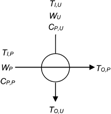
Heat exchanger.
When sizing the heat exchanger, the utility stream outlet temperature TO,U can be calculated from a recommended temperature approach [1], while an energy balance allows determining the mass flow of this stream, WU. The exchanger is governed by two energy conservation equations (Eqs. 1-2), a heat transfer relation (Eq. 3), and two additional equations (Eqs. 4-5).
| Q=WP(TI,P−TO,P) | (1) |
| Q=WU(TO,U −TI, U) | (2) |
| Q=UA∆TLMTD | (3) |
 |
(4) |
 |
(5) |
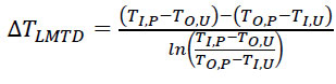
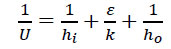
Where Q is the amount of energy exchanged, U is the overall heat transfer coefficient, A is the exchanger area, and ∆TLMTD is the logarithmic mean of the temperature differences. U is calculated from the thickness ε of the wall separating the currents in the exchanger, the thermal conductivity k of the metal, and the internal hi and external hO thermal convective coefficients. These last two coefficients are strongly dependent on the fluid flow and temperature conditions, so that in the early stages of design, it is impossible to know their value precisely. However, ranges of typical values of these coefficients can be found in engineering handbooks [40]. The ranges are denoted hi∈[hiMIN, hiMAX] and hO∈[hOMIN, hOMAX].
3.2. Heat Exchanger Sizing as a Decision Problem
In practice, the operation of the exchanger will likely involve a control system adjusting the flow of the utility stream to keep the outlet temperature of the process stream at a desired value or set-point (TO,PSP), as shown in Fig. (3). This would compensate for inaccuracies in the data used in sizing the exchanger.
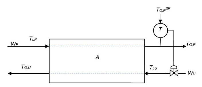
Actual heat exchanger setup.
The sizing problem consists of setting the area of the exchanger (A) and the maximum installed capacity of the utility stream (WU,MAX). An influence diagram of this decision is shown in Fig. (4). Circles represent uncertainties, squares stand for decisions, the circle with a double border means a deterministic calculation, and the hexagon represents the consequences. The finding of an optimal solution by using influence diagrams implies that the recommended design is chosen from a discrete set of alternatives and that the relevant probability distributions have been discretized. This is computationally convenient but can limit the quality of the solution found. More refined solution-searching approaches and simulation-based techniques for uncertainty propagation can be used to maintain the continuous nature of decisions and uncertainties, but these techniques would have increased the computational effort required to provide a solution.
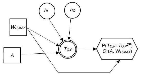
Influence Diagram for heat exchanger sizing.
The convective transfer coefficients hI and hO are the uncertainties of the problem, while A and WU,MAX represent the decisions. The arrows reaching the double-bordered circle indicate that when the mentioned four elements are known, the outlet temperature of the process stream, TO,P, is fixed. Consequences are outcomes that are important to the decision-maker, in this case, the probability that the process outlet temperature is at its set-point P(TO,P=TO,PSP) and the total cost CT, which depends on the design decisions. The decision model can be split into a factual model, based on equations 1 to 5, that calculates the probability distribution of TO,P given the decisions, and a value model providing a preference metric for consequences P(TO,P=TO,PSP) and CT. More precisely, the value model consists of a utility function that assigns a desirability value (utility) to the performance metric and exchanger size, the latter used as a proxy of cost. The expected utility of each alternative is calculated from its performance probability distribution and size. The chosen alternative is the one that gets the maximum expected utility.
3.2.1. Factual Model
The ranges of hI and hO are discretized as sets of N values [hI1= hIMIN, hI2,..., hIN=hIMAX] and [hO1= hOMIN, hO2,..., hON=hOMAX], with each value having the same probability 1/N. In the same way, it is assumed that the exchanger area and maximum installed utility stream capacity are to be chosen, respectively, from discrete sets of a and w alternatives A∈[A1,A2,...,Aa] and WU,MAX∈[WU,MAX1, WU,MAX2,..., WU,MAXw]. For a set of values hIi, hOk, Am, and WU,MAXn the algorithm shown in Fig. (5) calculates TO,P, and WU. The third step of Fig. (5) determines whether the configuration can keep the process stream outlet temperature at its set-point, first by calculating the maximum possible value of the logarithmic mean of the temperature differences (corresponding to a constant utility stream temperature and the outlet temperature of the process stream at its set-point). The minimum UA value, (UA)MIN, is determined from the heat needed to bring the process stream temperature to its set-point and the maximum value of the logarithmic mean of the temperature differences. If the specified value of UA is greater than (UA)MIN, the required utility current flow WU is calculated. If this WU value is less than the maximum installed capacity WU,MAXn, the outlet temperature of the process stream is set to TO,PSP, and the utility stream flow to WU. However, if the calculated value of WU is bigger than WU,MAXn or the value of UA is below (UA)MIN, the outlet temperatures of both streams TO,P, and TO,U are calculated with the flow of the utility stream at its maximum value WU,MAXn. In this case, the process stream outlet temperature cannot be kept at its set-point. So, given the parameters included in the top box of Fig. (5), the factual model allows the discretized probability distributions of the heat transfer coefficients to result in a probability distribution of the outlet stream tempera-
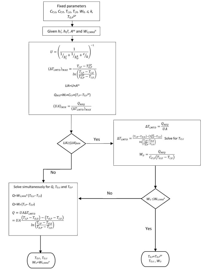
Algorithm for TO,P and WU calculation.
ture, as each combination of possibilities of the heat transfer coefficients produce an outlet temperature possibility, being the probability of said temperature the joint probability of the heat transfer coefficient possibilities. From this probability distribution, the performance metric (probability of maintaining the outlet temperature at its set point) is determined.
3.2.2. Value Model
To balance the objectives of keeping the outlet temperature of the process stream at its set-point and minimizing equipment cost, an additive value (or utility) function, Eq. (6), is assumed
| UG=kSP USP(P(TO,P=TO,PSP))+k$U$(CT) | (6) |
The weights kSP and k$ add up to one. USP takes a value of one for the greatest probability, among the alternative designs considered, of maintaining TO,P at its set point, PMAX(TO,P=TO,PSP), and takes the value of zero for the corresponding smallest probability PMIN(TO,P=TO,PSP), as shown in Eq. (7).
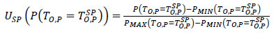 |
(7) |
The total cost CT, Eq. (8), is assumed to be linear with respect to the exchanger area and the maximum installed capacity of the utility stream
| CT=αA A + αW WU,MAX | (8) |
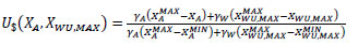
Where αA and αW are unitary cost factors. The function U$ is calculated based on CT according to Eq. (9):
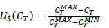 |
(9) |
Since the maximum cost CTMAX is that of the alternative specifying the greatest exchanger area and utility stream capacity (AMAX and WU,MAXMAX), and the minimum cost CTMIN is that of the alternative setting the minimum values of these decisions (AMIN and WU,MAXMIN), Eq. 9 can be rearranged as Eq. (10):
 |
(10) |
The selected design will be the one producing the highest expected value of the overall utility UG. Oversize percentages of area and utility stream capacity, XA and XWU,MAX, with respect to some base values AB and WU,MAXB, are defined as in Eqs. (11 and 12).
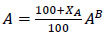 |
(11) |
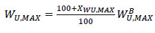 |
(12) |
For instance, if there is no overdesign in area, XA=0 and the area is equal to AB, while an overdesign of 200% (XA=200) corresponds to an area three times the size of AB. In terms of oversize percentage variables, U$ is expressed as Eq. (13):
 |
(13) |
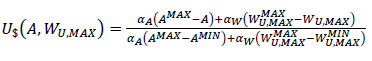
Where XAMAX, XAMIN, XWU,MAXMAX, and XWU,MAXMIN are the maximum and minimum overdesign percentages considered in the alternatives, respectively, for area and maximum flow capacity of the utility stream, while γA and γA are defined by Eqs. (14-15):
 |
(14) |
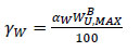 |
(15) |
Eq. 13 is rearranged to Eq. (16), so U$ can be calculated from the γA/γW ratio
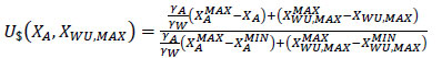 |
(16) |
The weights kSP and k$ depend on the decision maker´s trade-off between the temperature control objective and the equipment cost. To calculate these weights, a transition ∆TSP is defined as changing the lowest probability of keeping the process stream outlet temperature at its set point (among the considered design alternatives), to the corresponding highest probability. ∆TSP is formally stated in Eq. (17), where the arrow means “is changed into”
| ∆TSP: PMIN(TO,P=TO,PSP)→ PMAX(TO,P=TO,PSP) | (17) |
If the decision maker views this probability improvement as equivalent to a monetary amount Ce (Eq. 18):
| ∆TSP ∼ Ce | (18) |
Where “∼” means “is indifferent between”, and ∆CT is the breadth of the cost range among the alternatives, as in Eq. (19),
| ∆CT=αA(AMAX−AMIN) +αW (WU,MAXMAX− WU.MAXMIN) | (19) |
Then the weights can be derived from the indifference condition of Eq. (18), translated to
| kSP(USP(PMAX(TO,P=TO,PSP))−USP(PMIN(TO,P=TO,PSP)))=k$(U$(CTMIN)− U$(CTMIN + Ce)) | (20) |
Eq. (20) and kSP and k$ adding up to unity produce Eqs. (21 and 22):
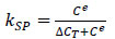 |
(21) |
 |
(22) |
3.3. Results and Discussion
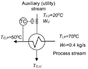
The exchanger shown in Fig. (6) is considered, where the objective is to cool a process stream of 0.4 kg/s, from 70°C to 50°C. For this purpose, a utility stream at 20°C is available.
Heat exchanger for a numerical example.
The heat capacities of the streams are CP,P=CP,U=4.180 kJ/kg K. With a minimum temperature approach of 30°C, the outlet temperature of the service stream is calculated as TO,U=40°C and its flow determined to be WU=0.4 kg/s. The exchanger metal wall thickness and thermal conductivity are ε=0.005 m and k=80 W/m K, while the convective coefficients hI and hO are known to be anywhere between 600 and 12'000 W/m2K [41].
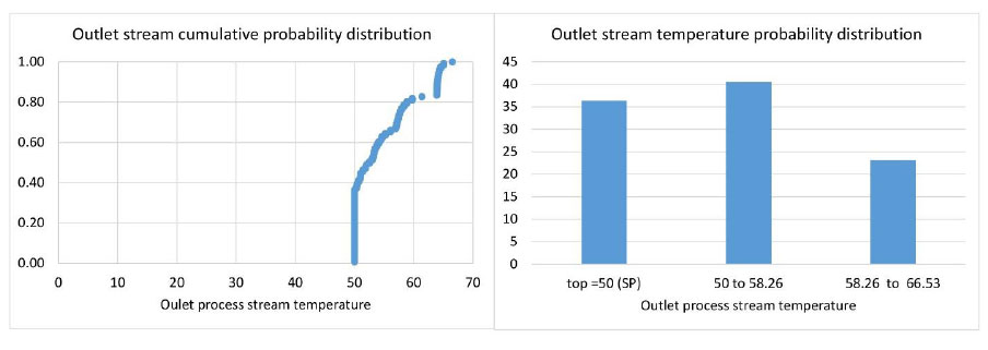
The base value of the area is calculated with the values of hI and hO at the middle of the range of possibilities (6300 W/m2K), which produces an area AB=0.423 m2. The base value of the maximum capacity of the utility stream is equal to the value calculated by the heat balance, WU,MAXB=0.4 kg/s.. By discretizing the range of hI and hO into eleven equally spaced points, each one with the same probability, and applying the algorithm in Fig. (5), the cumulative probability distribution of TO,P for the base design is calculated (Fig. 7). It is observed that the probability of getting the process stream to its set-point temperature is around 36%, while there is certainty of keeping this temperature below 68°C.
The probability distribution in Fig. (8) shows that for the base design, the most likely scenario is that the temperature will be greater than 50°C and below 58°C.
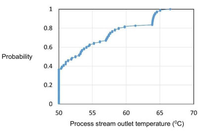
Cumulative probability distribution of TO,P for the base design.
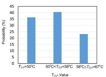
Probability distribution of TO,P for the base design.
Fig. (9) shows the effect of oversizing the area and maximum utility stream flow capacity on the probability of TO,P being at its set-point. It is observed that a 300% overdesign in both decisions achieves a probability of 91% of maintaining the outlet stream process temperature at its desired value. Fig. (10) shows the recommended overdesigns given kSP and γA/γW values. As kSP grows (to the right in the figure), maintaining the outlet stream temperature at its set-point becomes increasingly important compared with the equipment cost. Thus, moving to the right causes bigger overdesigns to be prescribed. Moving upward in the chart, the relative cost of heat exchanger area with respect to the cost of the utility stream maximum flow capacity (γA/γW) increases, so moving in this direction makes the model recommend smaller exchangers and larger provisions for the utility stream maximum flow.
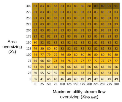
P(TO,P=TO,PSP) for different values of A and WU,MAX oversizing.
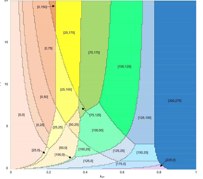
Recommended designs, shown as [XA, XWU,MAX] pairs, given kSP and γA/γW.
3.4. Excel Macro Interface for Heat Exchanger Sizing
The calculations described in Section 3.2 were coded in Visual Basic, to be run as a macro of Microsoft Excel. While several high-end mathematical software could have been used in developing and solving the model, a choice was made to use Excel in the current work, as it doesn’t require the purchase of a license in addition to that of MS-Office and is widely used by practicing engineers. The user opens an Excel file enabled to run macros and clicks on the “Calculate/show Interface” button (Fig. 11), which displays the main interface shown in Fig. (12). The data for the problem described in Section 3.3 appears as defaults in the relevant fields. Near the bottom left corner, the user can specify the limits of the ranges of thermal convective coefficients. By clicking “Calculate base dimensions”, the base values of exchange area and flow of the utility stream are calculated, using the middle range values of the coefficients.
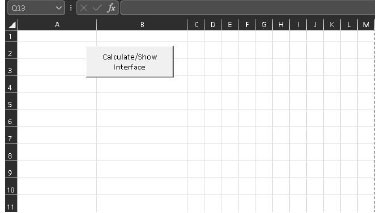
Initial program screen.
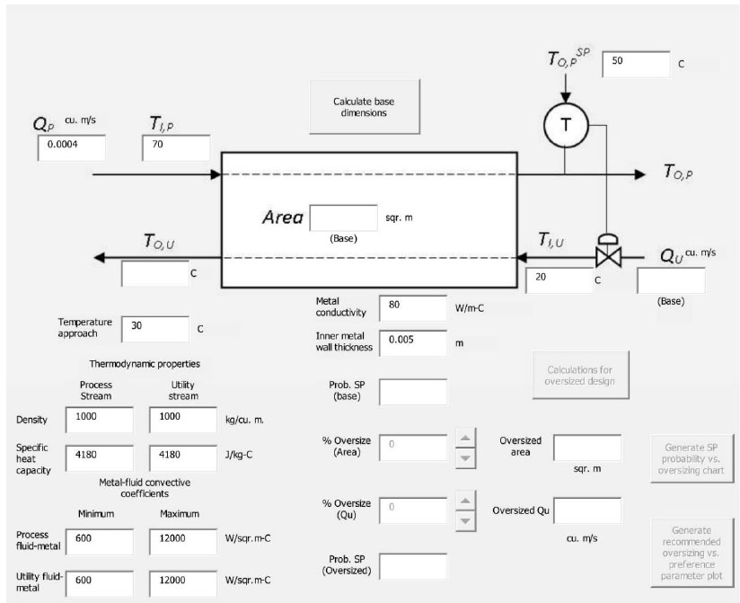
Main program interface.
A dialog box asks the user if the probability plots of the outlet process stream temperature are required. If so, the graphs of Fig. (13) are produced.
Once the base dimensions are calculated, the “Calculations for oversized design” button and the controls to specify oversizing percentages become active, as shown in Fig. (14) for a case in which a 50% overdesign is specified both in area and maximum flow of the utility stream. After clicking on the above-mentioned button, the augmented values appear in their respective boxes, as does the probability of maintaining the process stream at its set-point. A dialog box asks the user if a graph of probabilities for the augmented design is desired, in which case the graphs of Fig. (15) are produced.
Program output of base case TO,P probability charts.
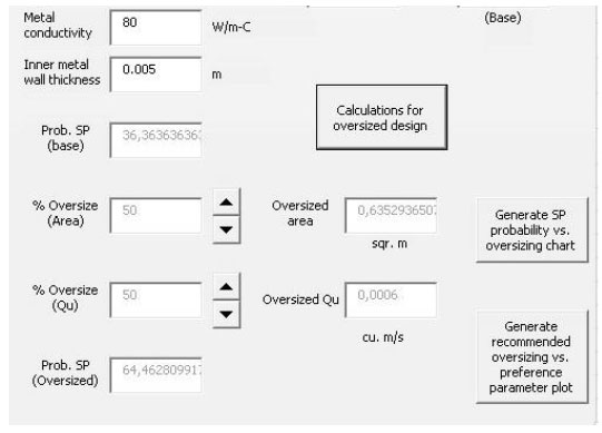
Controllers for specifying oversize percentages.
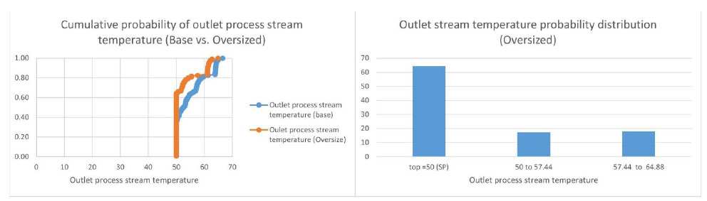
Program output of oversized design TO,P probability charts.
Finally, the button “Generate SP probability vs. oversizing chart” button produces a chart similar to Fig. (9), while the button “Generate recommended oversizing vs. preference parameter plot” produces one similar to Fig. (10).
CONCLUSIONS
Chemical process equipment design depends on physical parameters, some of which are not precisely known at the initial project stages. In said situations, equipment sizing can be stated as a decision-making problem under uncertainty and approached using Decision Analysis, as shown in this paper for the design of a heat exchanger. The decision model consists of a factual model that produces probability distributions of the process stream temperature given the design decisions, and a value model with weights measuring the importance of keeping this stream temperature at its set point relative to the design cost. In other words, the balance between the performance and cost is embodied in a utility function, whose weights are elicited from the engineer responsible for the design or provided directly by him. These weights are inherently subjective and depend on the specific application and the personal preference of the person purchasing the heat exchanger.
The main result is a graph with the recommended heat exchanger oversizing for different values of the weights used in the value function, which are intended to capture the decision-maker’s personal preferences. The proposed method was applied to a specific example and appeared to give reasonable results. While more tests are being carried out with data available in heat-exchanger literature, the approach still needs input and validation from practicing engineers, as they are the intended users of the model. Efforts in this direction are currently being taken. The decision process model acts on the probability distributions of the parameters, converting uncertain information of the heat transfer coefficients into a probability of maintaining the outlet temperature at its set-point. The empirical validation of this probability, however, would be very time-consuming to achieve, as, for example, it would require checking that the set point temperature is achieved in 9 out of 10 designs built for a 90% probability of keeping the target temperature. This would require checking the operation of a big enough sample size of the relevant functioning heat exchangers.
While the presentation can leave the impression that the model calculations are quite time-consuming for the objective of providing a preliminary heat exchanger size, the calculations can be automated as computer code, as done here in Visual Basic. The produced program, provided with a user-friendly interface, can be run in Microsoft Excel, thus avoiding the need to purchase specialized software licenses. The program developed here is aimed to be useful in the early stages of heat-exchanger design, in which the engineer relies on literature-reported ranges of typical values of the heat transfer coefficients and applies rule-of-thumb oversizing factors. The provided software shows the recommended oversized given the present uncertainty and the tradeoff between performance and cost. While there are several well-known heat-exchanger design computer packages, able to calculate the equipment thermal and mechanical designs, these are more adequate for equipment design at later project stages, when process parameters are known more precisely. Additionally, said packages do not show the dependence of the decision on the user preferences nor allow for uncertainty on parameters, as the program presented here.
AUTHORS’ CONTRIBUTIONS
It is hereby acknowledged that all authors have accepted responsibility for the manuscript's content and consented to its submission. They have meticulously reviewed all results and unanimously approved the final version of the manuscript.
AVAILABILITY OF DATA AND MATERIALS
The data supporting the findings of article is available through link: https://drive.google.com/file/d/1ttwqrX8W8 ecEH6U2f3JXWPKMSUG-Hhzu/view?usp=drive_link.
ACKNOWLEDGEMENTS
Declared none.