All published articles of this journal are available on ScienceDirect.

Dispersion Modelling of Air Pollutants from Industrial Point Sources
Authors Info & Affiliations
Abstract
Introduction
Industrial point sources emit a wide spectrum of air pollutants, posing significant threats to environmental quality and public health. Previous studies often focused on single pollutants or limited source types, reducing generalizability. This study addresses this gap by characterizing multiple pollutants gaseous emissions, particulate matter, and heavy metals across diverse industrial point sources and modelling their dispersion to assess spatial impacts on air quality.
Methods
Emissions were assessed from industrial facilities, including boilers, furnaces, kilns, and generators. Gaseous pollutants (HC, NOₓ, CO, VOC) were measured using an E8500 combustion analyzer, particulate matter (PM) was collected on quartz fiber filters with a high-volume air sampler and quantified gravimetrically, while heavy metals (Pb, As, Cd, Co, Zn) were analyzed via X-ray fluorescence (XRF). Dispersion modelling was conducted using AERMOD under five operational scenarios and ten pollutants.
Results
Dispersion modelling revealed notable heterogeneity in pollutant concentrations across scenarios. In Scenario 1 (boiler-only operation), predicted ground-level concentrations of Pb (147.292 μg/m³), As (30.476 μg/m³), and Cd (30.474 μg/m³) were high, while NOₓ (0.010 μg/m³) and CO (0.019 μg/m³) remained low, emphasizing the source-specific nature of emissions.
Discussion
The disproportionately high heavy metal concentrations highlight the need for targeted control of specific industrial processes, particularly boilers. Despite the reliability of AERMOD, dependence on a single dispersion model is a limitation.
Conclusion
This study presents a comprehensive emission inventory and dispersion modeling framework encompassing multiple industrial sources and pollutants. The results emphasize the critical role of diverse industrial activities in air quality degradation and offer a stronger scientific foundation for designing targeted emission control and mitigation strategies.
1. INTRODUCTION
Air pollution remains a pressing environmental and public health issue globally, and its effects are increasingly being felt in rapidly industrializing regions. It results in the release of harmful substances, including gases, particulate matter, and heavy metals into the atmosphere, which can lead to severe respiratory and cardiovascular health problems and damage to ecosystems [1-5]. Air pollution can also increase the risk of some cancers, such as lung cancer [6]. It has the potential to contribute to global warming, harm forests and agriculture, acidify lakes and streams [7, 8], and negatively impact the economy [9-14]. Air pollution involves a sequence of events from the generation of pollutants at the source and the release into the atmosphere, the transportation and transformation of these pollutants, and their effect on the ecosystem at large [15, 16]. While the causes of air pollution are both natural and anthropogenic, industrial emissions, particularly from point sources, are among the most significant contributors in urban and peri-urban environments [17-19].
In Nigeria, the expansion of the manufacturing sector over the past few decades has contributed significantly to the national GDP and employment [ 20 , 21 ], especially across industrial corridors in Lagos, Ogun, and other states. However, this industrial growth has come with environmental trade-offs. Industrial processes in the country frequently rely on fossil fuel combustion and emit a variety of air pollutants, including nitrogen oxides (NOx), sulfur dioxide (SO 2 ), carbon monoxide (CO), particulate matter (PM), volatile organic compounds (VOCs), and heavy metals such as lead (Pb), cadmium (Cd), and arsenic (As). These pollutants are released from production stacks, furnaces, kilns, boilers, and both diesel- and gas-powered generators that are common in Nigerian factories.
Understanding the natural and human causes of air pollution is critical for correctly estimating the health risks associated with air pollution and devising effective risk reduction measures [22]. Also, the dispersion behaviour of pollutants associated with air emission will guide the policy makers on stringent rules to put in place and policies to enact for air pollution mitigation measures. A significant portion of pollution comes from anthropogenic causes, which are also blamed for several dangerous air pollutants that can harm human health [23].
Combustion of fossil fuels, industrial operations, and motor vehicles are the three most frequent anthropogenic causes of air pollution [24-28]. Fuel combustion, industrial processes, transportation, and fugitive emissions are the principal sources of industrial air pollutants. Pollutants emitted by companies include carbon monoxide, nitrogen oxides, sulphur dioxide, particulate matter, and volatile organic compounds (VOCs) [29, 30], and hazardous air pollutants (HAPs), among others [31-33] depending on the nature of industrial activities. To generate electricity and heat, fossil fuels such as coal, oil, and natural gas are burnt, and this combustion process emits a range of products, which include air pollutants such as nitrogen oxides (NOx), carbon monoxide (CO), sulphur dioxide (SO2), and particulate matter (PM) [34-39].
Manufacturing processes such as chemical processing, paper manufacturing, and metal processing all emit air pollutants, notably volatile organic compounds (VOCs) [40-42]. Industrial point sources are stationary sources that emit pollutants directly into the atmosphere, such as factories and power plants [25, 43, 44]. There are two types of point sources: direct emissions, which are released directly into the atmosphere, and fugitive emissions, which are released indirectly into the atmosphere via fugitive or non-point sources such as tanks and pipelines. Pollutants emitted by point sources include volatile organic compounds (VOCs), sulphur dioxide (SO2), nitrogen oxides (NOx), particulate matter (PM), and carbon monoxide (CO) [34, 45-47]. Fugitive emissions are also an important source of industrial air pollutants, and these emissions are caused by leaks, spills, and other uncontrolled pollution releases [45, 46, 48]. Storage tanks, pressure containers, and process equipment are common industrial sources of fugitive emissions [49]. Pollutants emitted by these sources vary depending on the industry, but they might include VOC, CO, and HAP [50-52]. For decades, industrial point sources of air pollutants have been a major contributor to air pollution.
Nigeria's manufacturing industry has grown significantly in recent decades [53-57]. This expansion has been fuelled by a variety of causes, including increasing infrastructural investment, enhanced access to technology, and a more competitive corporate climate [53, 58-62]. Food and beverage, textiles and clothing, construction materials, chemicals and petrochemicals, metal products, machinery and equipment, and motor vehicles are the key industrial facilities in Nigeria [63-66].
Despite growing concerns, most air dispersion modelling and emission inventory from industrial point sources remain limited in scope. Previous studies have focused either on individual pollutants or emissions from a small number of industrial point sources or limited industries. In a study by [67], NO2 was the only pollutant from the 18 industries which dispersion modelling was conducted. This often neglects the combined effects of multiple pollutants from diverse industrial sources. This narrow focus fails to capture the broader impact of multiple pollutants emitted from various sectors operating simultaneously within industrial clusters. In another study, [68], SO2, PM10, and lead (Pb) were the pollutants considered from the industrial ambient area [68], conducted air dispersion modelling for SO2, PM2.5 in Kocaeli, Turkey, a region with industrial, traffic, and residential sources [69]. The study also used guassian dispersion modelling to predict SO2 ground-level concentration (GLC) from industrial sources, focusing on coal-fired power plants and a sponge iron plant in India [70].
In the region covered by this study, comprising clusters of food and beverage producers, petrochemical and chemical industries, metal fabrication plants, construction material manufacturers, and other facilities, air pollution is driven by a mix of high-emitting point sources. Yet, there has been a lack of detailed emission inventories and dispersion modelling that holistically accounts for both gaseous pollutants and heavy metals across multiple sources. To address this gap, this study conducted a comprehensive emission inventory and dispersion modelling of air pollutants from ninety (90) industrial facilities. These included 10 chemical and petrochemical plants, 7 construction material manufacturers, 29 food and beverage factories, 16 metal product industries, and 28 categorized as miscellaneous (e.g., cosmetics, plastics, packaging). Emissions were characterized using direct measurements and modelled using AERMOD to assess pollutant dispersion across various scenarios.
The aim of this study is to conduct dispersion modelling for gaseous pollutants and heavy metals from several industrial point sources. The objectives are:
- Characterize the pollutants into gaseous pollutants and heavy metals
- Perform air dispersion modelling to estimate their spread and concentration profiles in the surrounding environment.
2. MATERIALS AND METHODS
2.1. Study Area
Ogun State, a state in southwest Nigeria that was created in 1976 from the former Western State, is the focus of this research. According to the 2006 Census, Ogun State has a total area of 16,762.2 square kilometers and a population of roughly 5.8 million. The State is bordered to the north by the states of Oyo and Osun, to the south by Lagos state, to the east by Ondo state, and to the west by the Republic of Benin. It is located between 7°00′N 3°35′E [71].
The State has a variety of natural resources, including kaolin, bitumen, clay, granite, phosphate, and limestone. Ogun State is referred to as the industrial hub of Nigeria due to the large number of industrial estates that serve as home to both domestic and foreign industries, such as Agbara Estate, OPIC Agbara/Igbesa Estate, and Otta. Fig. (1) shows the map of the study area.
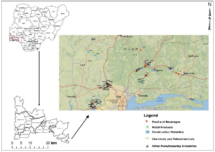
Map showing Ogun state with the identified types of manufacturing industries.
2.2. Gaseous Pollutants Characterization
Gaseous pollutants (NO X , CO, VOCs, and HC) were measured using the E8500 Plus portable emission analyzer, which employs non-dispersive infrared (NDIR) and electrochemical sensor technologies for precise detection. Prior to sampling, the instrument was calibrated daily using certified standard gases. The analyzer was calibrated prior to the field deployment.
The sampling probe of the analyser was inserted into the identified point sources, and measurements were taken for 2 minutes. All the measurements were taken while the identified point sources were working, and the average measurements were used for this study.
2.3. Heavy Metals Characterization
A high-volume air sampler, which consists of a 1-stage vacuum pump with an airflow volume of 12 cfm and a sampling probe, was used. The sampling probe consists of a filter holder where a Whatman 1 with a 25mm filter size is installed. The initial weight of the filters was recorded before and after sampling, and the weight difference was accounted for the total suspended particle (TSP). The concentration of TSP was calculated by dividing the weight difference by the volume of the air sampler. The volume was estimated by multiplying the high-volume sampler flow rate by the sampling duration of 2 minutes. Heavy metal concentrations in the particulate phase were determined using EDX3600B X-ray fluorescence spectroscopy (XRF). TSP-laden filters were collected and conditioned in a desiccator before analysis. The XRF method allowed for non-destructive multi-elemental analysis with high sensitivity.
To ensure quality and accuracy, field and laboratory blanks were run to correct for potential contamination. Calibration verification was performed at regular intervals. The Limit of Detection (LOD) and Limit of Quantification (LOQ) for each measured pollutant are presented in Table 1. For example, the LOD for NOX was 0.4 ppm, CO was 0.3 ppm, while that for Pb was 0.01 mg/m3 and As was 0.005 mg/m3. The overall analytical error was within ±10% for gaseous species and ±7% for heavy metals.
2.4. Total Suspended Particle Characterization
The total suspended particle (TSP) mass concentrations were estimated using the gravimetric method. This was determined by subtracting the initial average mass of the blank filter from the final average mass of the sampled filter. Filters were weighed using an analytical balance.
Since TSP/PM were estimated using gravimetric, the Limit of detection (LOD) and Limit of Quantification (LOQ) are not applicable to this in the same way they are for analytical techniques like X-ray fluorescence spectroscopy (XRF) or air sampler.
2.5 AIR DISPERSION MODELLING
To assess the spatial distribution and potential ground-level impacts of air pollutants emitted from industrial point sources, the AERMOD (American Meteorological Society/Environmental Protection Agency Regulatory Model) version 8.9.0 was used for the dispersion modelling. AERMOD is widely recognized for its robustness in simulating atmospheric dispersion in both rural and urban environments, especially under complex terrain and varying meteorological conditions.
2.5.1. Emission Source and Input Characterization
Key stack and source parameters, including height, exit diameter, exit temperature, and efflux velocity, were obtained from the industrial facilities surveyed or estimated using standard engineering formulas where direct measurements were unavailable. All emission sources were treated as point sources in the model.
2.5.2 Meteorological Data
Meteorological parameters for the year 2022 were processed using the AERMET meteorological pre-processor; the data were retrieved from the NASA website. Input variables included surface wind speed, wind direction, ambient temperature, atmospheric stability class, and mixing height. Data were sourced from the nearest synoptic meteorological station and complemented by on-site observations where available.
| Pollutant | Instrument Used | LOD | LOQ | Analytical Error (%) |
|---|---|---|---|---|
| NO X | E8500 Plus | 0.4 ppm | 1.2 ppm | ±10 |
| CO | E8500 Plus | 0.3 ppm | 0.9 ppm | ±10 |
| VOC | E8500 Plus | 0.05 ppm | 0.15 ppm | ±10 |
| HC | E8500 Plus | 0.03 ppm | 0.09 ppm | ±10 |
| Pb | XRF | 0.01 mg/m 3 | 0.03 mg/m 3 | ±7 |
| Cd | XRF | 0.005 mg/m 3 | 0.015 mg/m 3 | ±7 |
| As | XRF | 0.005 mg/m 3 | 0.015 mg/m 3 | ±7 |
| Co | XRF | 0.007 mg/m 3 | 0.021 mg/m 3 | ±7 |
| Zn | XRF | 0.01 mg/m 3 | 0.03 mg/m 3 | ±7 |
2.5.3 Terrain And Receptor Definition
Digital elevation data were incorporated through AERMAP, which refined surface elevations and hill features around the modelling domain. Receptors were distributed using a nested Cartesian grid system with finer resolution (100 m spacing) near source locations and coarser spacing at farther distances, extending up to 10 km from the emission source.
2.5.4 Model Configuration And Assumptions
The AERMOD simulation employed regulatory default settings, including rural dispersion coefficients, terrain effects, and building downwash features via the BPIP-PRIME algorithm. Stability classes were defined using surface data, with Pasquill-Gifford classification to determine atmospheric stability conditions. For the control pathway, 1-hour, 8-hour, 24-hour, and annual were the averaging time options considered for this study. To enhance realism, background concentrations from local air monitoring data were added to the model-predicted concentrations.
3. RESULTS AND DISCUSSION
For this study, five scenarios were considered, scenario 1, it was assumed that only boilers were working, scenario 2, it was assumed that only diesel powered generators were working, scenario 3, it was assumed that only gas powered generators were working, scenario 4, it was assumed that production stacks (kilns and furnaces were included) were working, scenario 5, it was assumed that all the industrial point sources were working concurrently which was considered as the worst case scenario. Tables 1 and 2 show the predicted concentrations for the identified pollutants.
3.1. Scenario 1: Boilers Only
In this scenario, where only boilers were operational, the highest 1-hour concentrations were observed for various pollutants. For arsenic, the concentration was 30.476 µg/m3, indicating a relatively high level of this toxic element. Cadmium exhibited a concentration of 30.474 µg/m3, which is in agreement with a study carried out by [72]. Lead reached a concentration of 147.292 µg/m3, indicating a significant presence of this heavy metal. Cobalt had a concentration of 10.396 µg/m3, suggesting the presence of this transition metal. Zinc exhibited a concentration of 7.517 µg/m3, indicating the presence of this element. Oxides of nitrogen had a concentration of 0.010 µg/m3. The results show the presence of heavy metals in large quantities in the boilers; these are detailed in Table 2.
A = Scenario 1
B = Scenario 2
C = Scenario 3
D = Scenario 4
E = Scenario 5
| As | Cd | Pb | Co | Zn | ||||||||||
|---|---|---|---|---|---|---|---|---|---|---|---|---|---|---|
| Averaging Period | Scenario | Concentration (µg/m3) | Averaging Period | Scenario | Concentration (µg/m3) | Averaging Period | Scenario | Concentration (µg/m3) | Averaging Period | Scenario | Concentration (µg/m3) | Averaging Period | Scenario | Concentration (µg/m3) |
| 1-Hour | A | 30.476 | 1-Hour | A | 30.474 | 1-Hour | A | 147.292 | 1-Hour | A | 10.396 | 1-Hour | A | 7.517 |
| B | 0.505 | B | 5.074 | B | 3.071 | B | 0.112 | B | 2.750 | |||||
| C | 0.000 | C | 0.002 | C | 0.723 | C | 0.100 | C | 16.698 | |||||
| D | 0.038 | D | 0.000 | D | 0.244 | D | 0.000 | D | 0.024 | |||||
| E | 27.254 | E | 24.156 | E | 90.158 | E | 11.854 | E | 8.177 | |||||
| 8-Hour | A | 12.869 | 8-Hour | A | 12.867 | 8-Hour | A | 71.843 | 8-Hour | A | 2.997 | 8-Hour | A | 2.685 |
| B | 0.386 | B | 2.349 | B | 2.351 | B | 0.052 | B | 0.952 | |||||
| C | 0.000 | C | 0.001 | C | 0.182 | C | 0.040 | C | 4.326 | |||||
| D | 0.010 | D | 0.000 | D | 0.066 | D | 0.000 | D | 0.006 | |||||
| E | 7.923 | E | 7.921 | E | 32.938 | E | 2.307 | E | 3.892 | |||||
| 24-Hour | A | 4.357 | 24-Hour | A | 4.356 | 24-Hour | A | 33.772 | 24-Hour | A | 1.066 | 24-Hour | A | 1.021 |
| B | 0.259 | B | 1.003 | B | 1.578 | B | 0.022 | B | 0.362 | |||||
| C | 0.000 | C | 0.001 | C | 0.061 | C | 0.019 | C | 2.630 | |||||
| D | 0.005 | D | 0.000 | D | 0.034 | D | 0.000 | D | 0.006 | |||||
| E | 3.496 | E | 3.494 | E | 12.040 | E | 0.814 | E | 1.701 | |||||
| Annual | A | 0.532 | Annual | A | 0.343 | Annual | A | 9.090 | Annual | A | 1.066 | Annual | A | 0.174 |
| B | 0.036 | B | 0.213 | B | 0.217 | B | 0.005 | B | 0.063 | |||||
| C | 0.000 | C | 0.000 | C | 0.006 | C | 0.004 | C | 1.003 | |||||
| D | 0.001 | D | 0.000 | D | 0.007 | D | 0.000 | D | 0.001 | |||||
| E | 0.332 | E | 0.327 | E | 1.213 | E | 0.077 | E | 0.579 | |||||
3.2. Scenario 2: Diesel Powered Generators Only
In this scenario, where only diesel-powered generators were operational, a range of pollutants was present in the atmosphere at varying concentrations. Table 2 shows the measured concentrations for diesel generators.
3.2.1. 1-Hour Averaging Period
From Fig. (2) arsenic, the concentration was 0.505 µg/m3, representing a relatively low level of this toxic element. Cadmium exhibited a concentration of 5.074 µg/m3. Lead reached a concentration of 0.097 µg/m3. Cobalt had a concentration of 0.112 µg/m3, indicating the presence of this transition metal. Zinc exhibited a concentration of 2.750 µg/m3, which is backed by a study carried out by [73]. These results indicate that diesel-powered generators emit air pollutants in excess, especially Cadmium and Zinc as compared to the other heavy metals in this scenario.
3.3. Scenario 3: Gas Powered Generator Only
3.3.1. 1-Hour Averaging Period
For Arsenic, the concentration was low. Cadmium exhibited a concentration of 0.002 µg/m3 as shown in Fig. (3). Lead reached a concentration of 0.723 µg/m3. Cobalt had a concentration of 0.100 µg/m3. Zinc exhibited a concentration of 16.698 µg/m3. Nitrogen oxides had a concentration of 0.005 µg/m3. Carbon monoxide reached a low concentration. Total Suspended Particles also had a concentration of 0.000 µg/m3, which shows that TSP is negligible. Volatile organic compounds exhibited a low concentration. Hydrocarbons had a concentration of 0.056 µg/m3. The results from gas-powered generators, as detailed in Table 3, indicated that these generators emit less air pollutants.
3.4. Scenario 4: Production Stacks (Kilns and Furnaces Included)
In this scenario, where production stacks, including kilns and furnaces, were operational:
3.4.1. 1-Hour Averaging Period:
Arsenic had a concentration of 0.038 µg/m3, indicating a relatively low presence of this toxic element. Cadmium exhibited a low concentration. Lead reached a concentration of 0.244 µg/m3. Cobalt had a low concentration. Zinc exhibited a concentration of 0.024 µg/m3. Nitrogen oxides had a low concentration. Carbon monoxide reached a low concentration as shown in Fig. (4). These results show that gas powered machinery (including the selected production stacks) emitted less gaseous pollutants, this is detailed in Table 3.
| NOx | CO | TSP | VOC | HC | |||||||||||
|---|---|---|---|---|---|---|---|---|---|---|---|---|---|---|---|
| Averaging Period | Scenario | Concentration (µg/m3) | Averaging Period | Scenario | Concentration (µg/m3) | Averaging Period | Scenario | Concentration (µg/m3) | Averaging Period | Scenario | Concentration (µg/m3) | Averaging Period | Scenario | Concentration (µg/m3) | |
| 1-Hour | A | 0.010 | 1-Hour | A | 0.019 | 1-Hour | A | 0.043 | 1-Hour | A | 0.005 | 1-Hour | A | 0.090 | |
| B | 0.008 | B | 0.097 | B | 0.000 | B | 0.021 | B | 0.001 | ||||||
| C | 0.014 | C | 0.005 | C | 0.054 | C | 0.000 | C | 0.056 | ||||||
| D | 0.000 | D | 0.000 | D | 0.000 | D | 0.000 | D | 0.070 | ||||||
| E | 0.011 | E | 0.073 | E | 0.034 | E | 0.027 | E | 0.070 | ||||||
| 8-Hour | A | 0.003 | 8-Hour | A | 0.005 | 8-Hour | A | 0.018 | 8-Hour | A | 0.002 | 8-Hour | A | 0.035 | |
| B | 0.002 | B | 0.036 | B | 0.000 | B | 0.010 | B | 0.000 | ||||||
| C | 0.005 | C | 0.001 | C | 0.014 | C | 0.000 | C | 0.015 | ||||||
| D | 0.000 | D | 0.000 | D | 0.000 | D | 0.000 | D | 0.018 | ||||||
| E | 0.004 | E | 0.040 | E | 0.011 | E | 0.012 | E | 0.032 | ||||||
| 24-Hour | A | 0.001 | 24-Hour | A | 0.002 | 24-Hour | A | 0.006 | 24-Hour | A | 0.001 | 24-Hour | A | 0.015 | |
| B | 0.001 | B | 0.018 | B | 0.000 | B | 0.007 | B | 0.000 | ||||||
| C | 0.003 | C | 0.001 | C | 0.005 | C | 0.000 | C | 0.008 | ||||||
| D | 0.000 | D | 0.000 | D | 0.000 | D | 0.000 | D | 0.007 | ||||||
| E | 0.002 | E | 0.024 | E | 0.005 | E | 0.004 | E | 0.012 | ||||||
| Annual | A | 0.000 | Annual | A | 0.000 | Annual | A | 0.001 | Annual | A | 0.000 | Annual | A | 0.005 | |
| B | 0.000 | B | 0.004 | B | 0.000 | B | 0.001 | B | 0.000 | ||||||
| C | 0.001 | C | 0.000 | C | 0.001 | C | 0.000 | C | 0.001 | ||||||
| D | 0.000 | D | 0.000 | D | 0.000 | D | 0.000 | D | 0.002 | ||||||
| E | 0.001 | E | 0.007 | E | 0.001 | E | 0.000 | E | 0.002 | ||||||
3.5. SCENARIO 5: All Industrial Point Sources Concurrently (Worst Case Scenario)
In this worst-case scenario, where all industrial point sources were operational simultaneously as detailed in Table 4:
3.5.1. 1-Hour Averaging Period:
Arsenic had a concentration of 27.254 µg/m3. Cadmium exhibited a concentration of 24.156 µg/m3. Lead reached a concentration of 90.158 µg/m3. Cobalt had a concentration of 11.854 µg/m3. Zinc exhibited a concentration of 8.177 µg/m3. Nitrogen oxides had a concentration of 0.011 µg/m3. Carbon monoxide reached a concentration of 0.027 µg/m3. From Fig. (5) total Suspended Particles had a concentration of 0.034 µg/m3. From Table 5, the gaseous pollutant, hydrocarbon, and volatile organic compounds from diesel-powered generators are in large quantities due to incomplete combustion of diesel, high combustion temperatures, and other factors.
The dispersion modelling results across the five scenarios revealed notable differences in pollutant concentrations, largely influenced by fuel type (diesel vs. gas), generator technology, and averaging periods (1-hour to annual).
3.5.1.1. Scenario 1
Scenario 1, which represents emissions from large-scale diesel-powered generators, showed the highest pollutant concentrations across the scenarios, particularly under short-term exposure conditions. Heavy metals such as arsenic, cadmium, and lead reached maximum 1-hour average concentrations of 12.869 µg/m 3, 12.867 µg/m 3, and 71.843 µg/m 3, respectively. These values significantly exceed background levels and, in the case of lead, even the WHO annual guideline value of 0.5 µg/m 3 was surpassed (0.343 µg/m 3). This suggests long-term environmental persistence and public health implications.
Gaseous pollutants, including hydrocarbons and carbon monoxide, were also present at notable levels, with hydrocarbons at 0.090 µg/m3 and CO at 0.019 µg/m 3 for the 1-hour average. Though these concentrations were below acute exposure limits, their presence indicates incomplete combustion, a common characteristic of diesel fuel. Notably, hydrocarbons’ potential to contribute to ozone formation and secondary organic aerosol (SOA) generation necessitates regulatory concern.
| Pollutant (µg/m3) | ||||||||||
|---|---|---|---|---|---|---|---|---|---|---|
| Boiler | HC | CO | NOX | VOC | PM | Co | Zn | As | Pb | Cd |
| B1 | 193.460 | 56.110 | 233.180 | 0.000 | 471.140 | 0.000 | 0.286 | 0.000 | 0.000 | 0.000 |
| B2 | 62.990 | 0.000 | 175.130 | 0.000 | 73.620 | 5.520 | 1.058 | 12.689 | 0.000 | 1.124 |
| B3 | 50.990 | 58.030 | 103.620 | 0.000 | 323.910 | 0.000 | 0.272 | 0.222 | 1.015 | 0.000 |
| B4 | 13.500 | 198.690 | 129.020 | 0.000 | 12323.320 | 0.000 | 1.843 | 0.000 | 0.000 | 0.000 |
| B5 | 41.990 | 95.430 | 450.810 | 0.000 | 441.700 | 0.000 | 0.274 | 0.000 | 0.000 | 0.000 |
| B6 | 44.990 | 85.890 | 334.750 | 0.000 | 29.450 | 5.106 | 1.377 | 21.923 | 0.197 | 0.978 |
| B7 | 14948.670 | 8.230 | 121.250 | 906.730 | 235.570 | 0.000 | 0.844 | 0.561 | 2.553 | 0.000 |
| B8 | 52.790 | 0.000 | 191.730 | 0.000 | 9422.850 | 0.000 | 0.269 | 2.668 | 52.703 | 0.000 |
| B9 | 95.980 | 85.890 | 164.780 | 0.000 | 309.190 | 0.028 | 0.207 | 2.055 | 36.329 | 0.000 |
| B10 | 46.490 | 130.170 | 524.400 | 0.000 | 279.740 | 0.011 | 0.283 | 3.066 | 67.628 | 0.000 |
| B11 | 287.940 | 0.000 | 244.590 | 0.000 | 294.460 | 0.000 | 0.280 | 2.667 | 56.170 | 0.000 |
| B12 | 15.000 | 206.140 | 346.120 | 0.000 | 176.680 | 0.004 | 0.334 | 1.213 | 15.821 | 0.000 |
| B13 | 53.990 | 41.990 | 204.170 | 3.970 | 323.910 | 0.030 | 0.319 | 0.000 | 0.000 | 0.000 |
| B14 | 359.920 | 2.740 | 205.190 | 0.000 | 515.310 | 0.000 | 4.271 | 0.679 | 4.589 | 0.000 |
| B15 | 930.390 | 1742.230 | 141.990 | 3.970 | 530.040 | 0.018 | 0.193 | 0.161 | 0.791 | 0.000 |
| B16 | 179.960 | 6.870 | 0.000 | 9.240 | 235.570 | 0.000 | 0.286 | 0.154 | 0.607 | 0.000 |
| B17 | 137.970 | 944.410 | 520.230 | 37.000 | 588.930 | 0.000 | 0.265 | 0.188 | 0.823 | 0.000 |
| B18 | 371.910 | 332.490 | 72.530 | 0.000 | 29.450 | 0.000 | 0.271 | 0.242 | 1.640 | 0.000 |
| B19 | 176.960 | 0.000 | 132.660 | 0.000 | 397.530 | 0.000 | 0.274 | 0.223 | 1.420 | 0.000 |
| B20 | 29.990 | 95.430 | 329.550 | 0.000 | 456.420 | 0.000 | 0.258 | 0.207 | 1.470 | 0.000 |
| B21 | 11.990 | 4.960 | 200.000 | 0.000 | 147.230 | 0.079 | 0.876 | 0.731 | 3.589 | 0.000 |
| Pollutant (µg/m3) | ||||||||||
|---|---|---|---|---|---|---|---|---|---|---|
| Diesel Generator | HC | CO | NOX | PM | VOC | Co | Zn | As | Pb | Cd |
| DG1 | 6.000 | 31.690 | 2632.300 | 313.910 | 16.375 | 0.000 | 0.311 | 0.000 | 0.000 | 0.000 |
| DG2 | 296.930 | 129.410 | 1289.210 | 206.120 | 349.781 | 0.000 | 2.968 | 0.060 | 0.249 | 0.000 |
| DG3 | 485.890 | 148.500 | 1652.960 | 353.360 | 285.630 | 0.000 | 0.850 | 0.714 | 4.346 | 0.000 |
| DG4 | 698.850 | 356.160 | 594.840 | 426.970 | 9.471 | 0.000 | 0.265 | 0.000 | 0.000 | 0.000 |
| DG5 | 1574.650 | 606.960 | 555.490 | 206.120 | 3.143 | 0.000 | 0.318 | 0.000 | 0.000 | 0.000 |
| DG6 | 305.930 | 84.370 | 2391.850 | 117.790 | 180.351 | 0.000 | 0.247 | 0.041 | 0.173 | 0.000 |
| DG7 | 188.960 | 122.540 | 3155.640 | 14.720 | 20.613 | 0.000 | 0.186 | 0.000 | 0.000 | 0.001 |
| DG8 | 959.790 | 199.640 | 2556.620 | 323.910 | 32.781 | 0.000 | 0.221 | 0.000 | 0.007 | 0.000 |
| DG9 | 41.990 | 214.920 | 1736.910 | 353.360 | 2.209 | 0.000 | 0.200 | 0.000 | 0.008 | 0.000 |
| DG10 | 50.990 | 1264.680 | 1116.130 | 117.790 | 11.043 | 0.000 | 0.248 | 0.000 | 0.000 | 0.000 |
| DG11 | 1073.760 | 512.280 | 2665.440 | 73.620 | 111.727 | 0.000 | 0.257 | 0.000 | 0.000 | 0.000 |
| DG12 | 26.990 | 66.800 | 1409.400 | 235.570 | 11.570 | 0.000 | 0.224 | 0.000 | 0.000 | 0.001 |
| DG13 | 38.990 | 26.720 | 3245.800 | 1752.060 | 12.148 | 0.000 | 0.264 | 0.000 | 0.000 | 0.002 |
| DG14 | 26.990 | 142.380 | 2674.770 | 206.120 | 2.945 | 0.174 | 0.000 | 0.000 | 0.000 | 7.908 |
| DG15 | 290.930 | 86.270 | 3567.050 | 618.370 | 19.877 | 0.000 | 0.229 | 0.000 | 0.000 | 0.000 |
| DG16 | 89.980 | 2143.440 | 3527.690 | 216.120 | 29.214 | 0.000 | 0.252 | 0.000 | 0.000 | 0.000 |
| DG17 | 371.910 | 214.150 | 3192.940 | 368.080 | 25.350 | 0.000 | 0.305 | 0.000 | 0.000 | 0.000 |
| DG18 | 29.990 | 252.710 | 1434.270 | 206.120 | 11.477 | 0.000 | 0.578 | 0.000 | 0.000 | 0.000 |
| DG19 | 98.980 | 297.750 | 2024.980 | 220.850 | 28.710 | 0.000 | 0.697 | 0.000 | 0.000 | 0.000 |
| DG20 | 161.960 | 932.190 | 7072.980 | 235.570 | 111.727 | 0.000 | 0.236 | 0.000 | 0.000 | 0.000 |
| DG21 | 380.910 | 142.380 | 2181.490 | 235.570 | 11.570 | 0.000 | 0.265 | 0.000 | 0.000 | 0.001 |
| DG22 | 53.990 | 125.590 | 2300.660 | 265.020 | 12.148 | 0.000 | 0.267 | 0.000 | 0.005 | 0.000 |
| DG23 | 116.970 | 272.560 | 1193.860 | 309.190 | 2.945 | 0.000 | 0.000 | 0.000 | 0.000 | 0.000 |
| DG24 | 44.990 | 83.600 | 4020.960 | 795.050 | 19.877 | 0.000 | 0.000 | 0.000 | 0.000 | 0.000 |
| DG25 | 1151.740 | 232.100 | 938.920 | 161.960 | 29.214 | 0.000 | 0.000 | 0.000 | 0.000 | 0.000 |
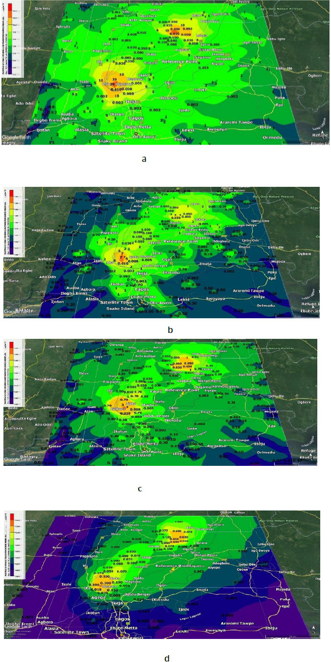
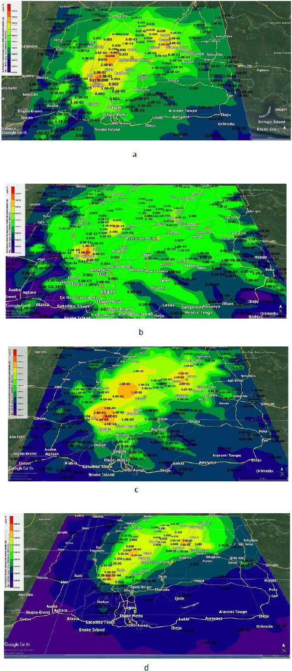
Contour plots of arsenic concentration for scenario 5 (a-1-hr, b-8-hr, c-24-hr, d-Annual)
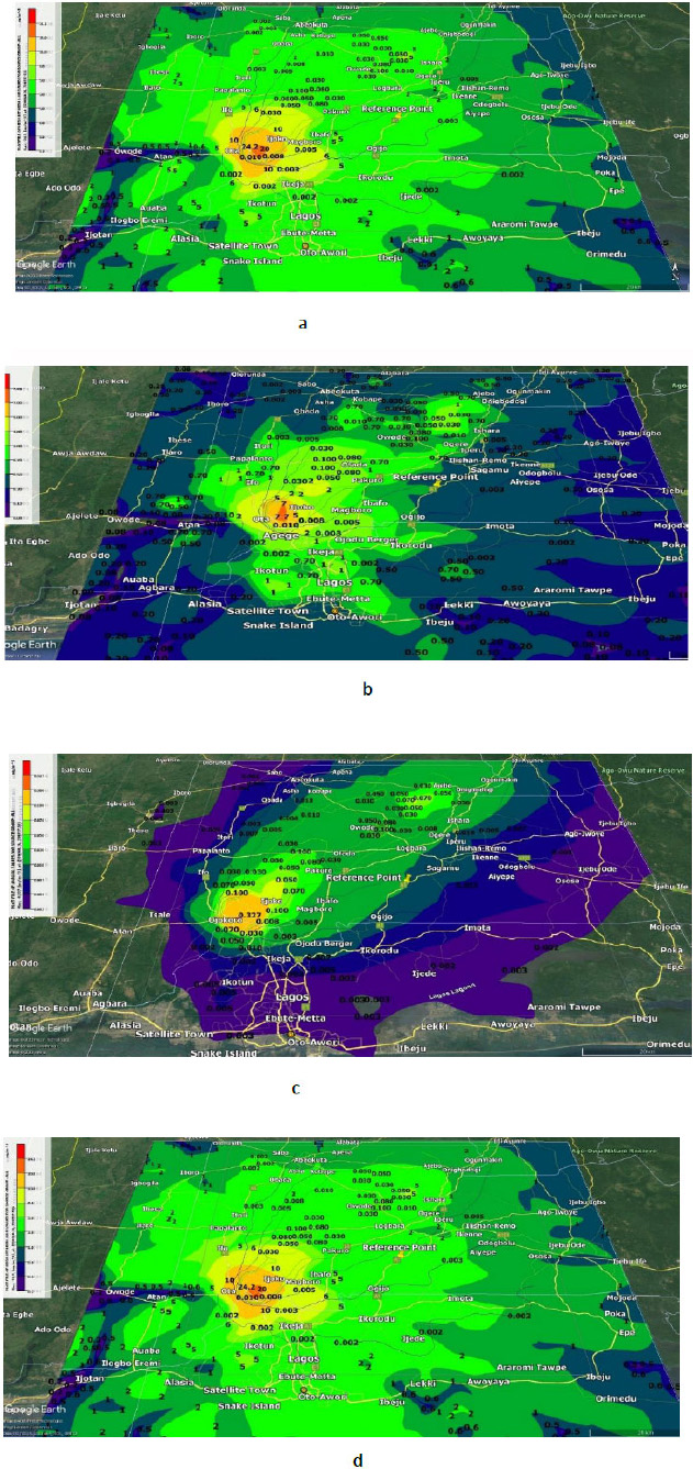
Contour plots of cadmium concentration for scenario 5 (a-1-hr, b-8-hr, c-24-hr, d-Annual).
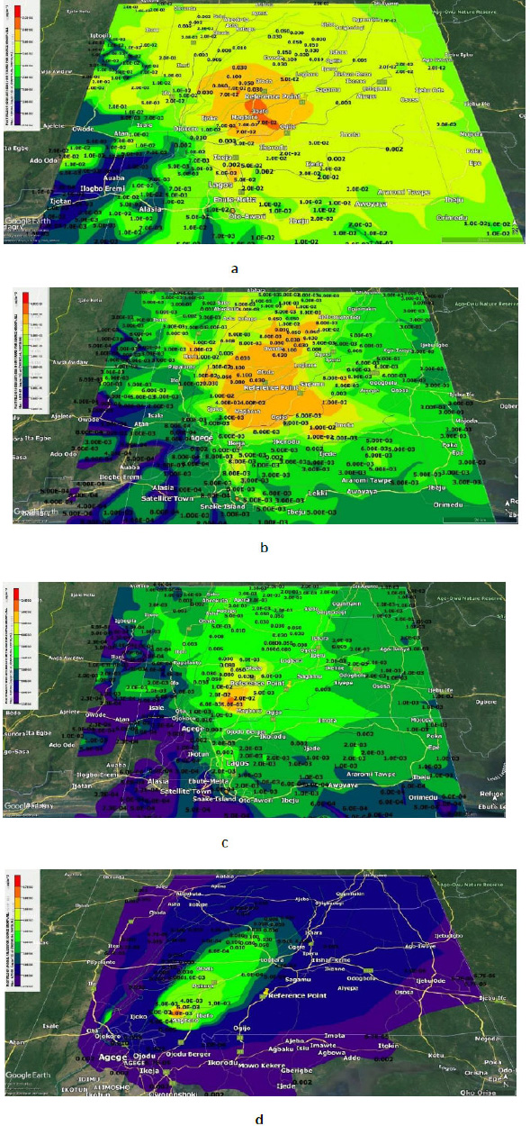
Contour plots of carbon monoxide concentration for scenario 5 (a-1-hr, b-8-hr, c-24-hr, d-Annual).
Contour plots of total suspended particle concentration for scenario 5 (a-1-hr, b-8-hr, c-24-hr, d-Annual).
3.5.1.2. Scenario 2
In this scenario, emissions stemmed from a combination of small diesel generators commonly used in residential or small commercial settings. While total emissions were lower than Scenario 1, pollutants such as volatile organic compounds still reached 1-hour average concentrations of 0.021 µg/m 3, and oxides of nitrogen concentrations were detectable but reduced compared to Scenario 1. These lower values reflect the smaller combustion volumes, but incomplete combustion and poor fuel-air mixing remain concerns. Studies have shown that such generators, due to poor maintenance and fuel inefficiency, can still contribute significantly to local air pollution and photochemical smog formation [74 ].
3.5.1.3. Scenario 3
Scenario 3, involving gas-powered generators, showed the lowest emissions across all pollutants and averaging periods. Most pollutants had annual average concentrations below 0.002 µg/m 3, and even the highest 1-hour average values remained minimal. For instance, lead and cadmium were below detection limits, while hydrocarbon was 0.015 µg/m 3. These findings confirm the cleaner combustion profile of natural gas compared to diesel, which aligns with results from [75], who documented substantially lower emissions from gas-fired power units. Nevertheless, low but detectable volatile organic compounds and hydrocarbon concentrations in this scenario suggest that gas combustion is not entirely free of environmental concerns.
3.5.1.4. Scenario 4
Scenario 4 evaluated emissions from backup and emergency generators operated intermittently. Despite lower annual pollutant concentrations, short-term (8-hour average) spikes were evident, especially for lead (lead: 0.066 µg/m 3), volatile organic compounds (0.017 µg/m 3), and oxides of nitrogen (0.032 µg/m 3). These episodic surges may cause transient local air quality deterioration, especially in enclosed or high-density areas. These findings underscore the environmental significance of even non-continuous emission sources, particularly in urban environments where dispersion is limited.
3.5.1.5. Scenario 5
The worst-case scenario was modelled to reflect peak emission conditions from high-output industrial diesel generators under minimal dispersion settings. The highest pollutant levels were recorded in this scenario. For instance, Arsenic reached 7.923 µg/m3 (8-hour average), lead was 65.241 µg/m 3, and cadmium was 11.109 µg/m 3. Hydrocarbons peaked at 0.070 µg/m3, and volatile organic compounds reached 0.027 µg/m3. These values were consistent with literature reporting extreme pollutant emissions from large-scale diesel generator banks [76]. This scenario highlights the compounded risk from both heavy metals and organic gaseous pollutants in dense industrial areas lacking adequate ventilation or emission control technologies.
CONCLUSION
In this study, we investigated ten air emissions emanating from seventy-three (73) industrial point sources. The emission inventory was taken, and the predicted concentrations show the dispersion behaviour of the identified pollutants. Industrial boilers have the highest amount of carbon monoxide (CO) with ranges of 0 -1742.23 µg/m3±411.06 and total suspended particles (TSP) of 29.45 - 12323.32 µg/m3±3214.67. The study can serve as a guide for air emissions regulatory bodies and policy makers in their decision-making toward zero carbon emissions.
AUTHORS’ CONTRIBUTIONS
A.J.A: Conceptualization, Methodology, Data Curation, Formal Analysis, Writing, Visualization – Original Draft. J.A.S.: Supervision, Project Administration, Writing – Review & Editing. D.O.O.: Methodology, Data Collection, Visualization, Investigation. O.A.A.: Validation, Resources, Writing – Review & Editing. O.S.: Data Curation, Formal Analysis, Visualization. A.R.L.: Literature Review, Writing – Review & Editing. E.O.O.: Validation, Technical Support. All authors have read and approved the final version of the manuscript.