All published articles of this journal are available on ScienceDirect.

A Decision Analytic Approach for Inspecting Leaking Hydraulic Distribution Systems that Relies on Bayesian Updating of Limited Information
Authors Info & Affiliations
Abstract
Introduction/Objective
When a liquid distribution system, particularly Hydraulic Distribution Systems, composed of several sections, experiences a leak, limited prior knowledge is available regarding which section is leaking. Longer sections have a higher likelihood of leaking, whereas larger fractures tend to occur in sections with greater diameter and higher pressure. This study proposes a procedure to update this information based on a gross observation of the leak size. The goal is to support strategic planning of leak detection by accounting for the time required to inspect each section.
Methods
The procedure employs a Decision Analysis approach to the problem, utilizing simulation and a basic hydraulic model. The available information is classified into “a priori” (available before the leak appears) and “a posteriori” (a Bayesian update of the a priori information after observing the flow rate at the end of the system). The data is used in decision trees that select the inspection sequence, minimizing the expected value of the total volume of lost fluid.
Results
A three-section hydraulic distribution system is analyzed numerically in a case study. When based on a priori information, the recommended review sequences begin with longer and higher-pressure sections. In contrast, when based on updated information, high-pressure sections are reviewed first if the leak is believed to be significant, while low-pressure ones are favored when the leak appears to be minor. Generally, the procedure recommends reviewing the first sections that can be checked swiftly.
Discussion
As the results are consistent with expectations for the system behavior, the procedure successfully leverages the available information and observations. As the presented approach uses a basic hydraulic model, it can be readily used by engineers without extensive computational resources.
Conclusion
A Decision Analytic perspective can be used to leverage available knowledge and modelling tools, whether the former is scarce or the latter basic, to improve leak detection in a multi-section hydraulic system, accounting for the time required to review each section.
1. INTRODUCTION
The problem of locating leaks in hydraulic distribution networks has been approached by several research groups. Most published methods are computationally intensive, use refined fluid-mechanics models, or require either parameter values that are not usually measured online or pressures and flows at many sites. In real life, as is the case with tap water distribution systems, measurements are made only in a handful of places and with limited accuracy. This work puts forward a more down-to-earth approach that begins by quantifying the initial knowledge regarding the potential leak location (denoted “a priori” information). It then applies simulation and a basic hydraulic model to update these beliefs based on an observation related to the leak size once it occurs, and uses the updated knowledge to guide the search for the leak. The approach is based on Decision Analysis, a discipline that supports decision-making under uncertainty [1]. The objective of Decision Analysis is to maximise the utility of the information available to the decision-maker at the time a decision needs to be made. By using these tools, the user is guaranteed to make a “good decision” in the sense that it complies with a set of axioms for rational decision making.
Following the description of the proposed methodology, the approach is numerically applied to a simple three-section piping system for demonstration. This work distinguishes itself from previously reported algorithms for leak searching in fluid distribution networks by adopting a Decision-Analytic approach and explicitly using a priori information. Additionally, it is more directly applicable than other algorithms, whose complexity limits their widespread use by hydraulic engineers without access to substantial computational resources.
1.1. Literature Review
Published research on algorithms for leak location in hydraulic networks can be divided into two categories: those based on pressure and flow gauges, and those that measure other variables. Among the former are Anfinsen and Aamo [2], who developed a model based on hyperbolic equations to detect the location and size of leaks; Blesa et al. [3] used a linear model with variable parameters and EPANET software to estimate the location of leaks by comparing estimated and actual pressure heads; Adachi et al. [4] estimated leak locations by minimizing the difference between measured and modeled pressures and flows, and Ruzza et al. [5] applied Kalman filtering to estimate leak locations. The inclusion of uncertainty to the leak location problem is presented by Liao et al. [6] who applied frequency response analysis and deep learning, by Morosini et al. [7] and Costanzo et al. [8] who applied model calibration, by Tylman et al. [9] who developed an automated system for detecting dielectric fluid leaks from buried cables using Bayesian networks and artificial intelligence, and by Malekpour et al. [10] and Lazhar et al. [11] who used an inverse transient analysis model and genetic algorithms to detect leaks in oil lines, taking into account the viscoelasticity of the pipe walls. Recently, Moosavian et al. [12] applied a neuro-fuzzy inferential model for leak location, aiming to minimize the number of head measurements needed, and Vorathin et al. [13] compared sensor types for leak location purposes in low-pressure gas distribution networks.
Regarding methods for locating fluid leaks, measuring variables additional to pressures and flows, Tariq et al. [14] suggest using accelerometers to detect leaks in water networks through neural networks and decision trees, while Wang et al. [15], within the framework of the homogeneous transformation theory, combined magnetic markers and internal detectors. On the use of sound wave propagation measurements, Zeng et al. [16] proposed using a “coherence-gram” to locate leaks in buried pipes, Scussel et al. [17] used acoustic correlators and Monte Carlo simulation to incorporate the effect of the uncertainties in pipe geometry and material properties on the propagation rate of the noise provoked by the leak while Li et al. [18] resorted to Fourier transformations for analyzing the acoustical waves produced by the lost fluid.
Recently, several research groups have published algorithms that use acoustic gauges (hydrophones) to detect leaks in water distribution networks. Satterlee et al. [19] coupled acoustic measurements with vibration meters to feed a neural network, Sitaropoulos et al. [20] and Uchendu et al. [21] applied, respectively, multifractal analysis and a multipath model to the task, while the simultaneous location of several leaks is discussed by Zeng et al. [22] and Liu et al. [23]. Additionally, Xu et al. [24] dealt with locating leaks in hot water networks, Islam et al. [25] employed thermal images and geo-acoustic probes for their leak searching algorithm, Sohn et al. [26] showed the operation of hydrophones tagged to fire hydrants to realistically test their frequency analysis-based leak location algorithm and Jacobsz [27] suggested the installation of fiber optic cables close to buried water pipes, to detect the temperature and stress changes provoked by a leak. Regarding leaks in gas distribution systems, Xiao and Li [28] compared acoustic techniques for detecting leaks in complex low-pressure networks, while Ali et al. [29] applied empirical model decomposition and K-clustering to improve the signal-to-noise ratio of the acoustic measurements.
There are also studies focused on optimally locating sensors in fluid distribution networks to better detect potential leaks. Li et al. [30] developed a clustering algorithm to optimally place pressure sensors in water distribution networks for leak detection, Hu et al. [31] applied multi-objective optimization to locate pressure sensors considering the severity of leaks in different places, while Goulet et al. [32] used model falsification to optimize the position of a minimum number of flow velocity meters.
Finally, regarding the planning of inspections of the network, Mancuso et al. [33] applied the Robust Portfolio Modeling approach and multi-attribute risk-based value theory to schedule inspections and maintenance operations in underground pipelines. Khaleel and Simonen [34] analyzed the selection of ultrasonic inspection strategies and inspection intervals to maximize tube reliability, and Ossai et al. [35] addressed inspection and repair decisions for lines prone to internal corrosion, using Markov chains and Monte Carlo simulation.
None of the reported procedures applies Decision Analysis, in the sense introduced by Howard [1], to the leak location problem. Additionally, previous published research does not consider subjective knowledge relative to the pipes' conditions nor use it to obtain “a posteriori” probability distributions, which are used to solve a decision problem under uncertainty to produce a plan to locate the leak. Finally, the application of the procedure shown here is much simpler than the methods previously reported, which, due to their mathematical and computational complexity, are not feasible for most engineers supervising hydraulic networks, given the time and tools available.
2. METHODS
It is assumed that the characteristics (e.g., pipe lengths, diameters, elevations, nominal inlet and outlet flows, pressures) of each section in the hydraulic distribution network are known, as are the times required to inspect each section for leaks. The objective of the procedure is to select the review sequence that minimizes the expected value of the amount of liquid lost until the leaking section is identified. It comprises the following steps:
Elicitation of a priori knowledge. The beliefs about which sections are more (or less) likely to show a leak, and which sections are likely to show bigger (or smaller) cracks, are quantified by probability distributions. For example, if all points along the pipe have the same probability of fracturing, then the leak position is uniformly distributed over the pipe's length. It can be assumed that larger holes are more likely to occur in sections with a larger diameter. The operator’s beliefs about leak likelihood in each section, considering factors such as pipe thickness, material, corrosion, age, and a higher propensity for leaks at bends or connections, are expressed through subjective probability distributions. The elicitation of subjective probability distributions can be performed using a “probability wheel” [1]. For example, an engineer may be asked whether, upon learning that a leak has occurred, they would consider it more likely to occur in certain sections of the network than others, or whether leaks are more probable at bends compared to straight sections of the pipeline. When a leak occurs, it is likely to produce noticeable effects, such as a diminished outlet flow. Using a basic hydraulic model (i.e., based on the Bernoulli equations) and simulation, the probability distributions of the leak location and size are used to derive the probability distribution of the outlet flow when the leak occurs. The probability distribution of the outlet flow conditional on the leak being in a particular section is also derived for all pipe sections.
(A) Defining the observation to be taken when the leak happens. For example, if the observation is defined as “the leak is big/small”, this can be made precise by describing an event “the outlet flow (i.e., the flow reaching the end of the network) is below/above a threshold value”.
(B) The decisions and uncertainties in the sequential review of the sections are set up in a decision tree. The tree begins with the event of whether the outlet flow is above or below a threshold value. Following this event, decisions (which section to review) and uncertain events (whether the leak was found in the selected section) are intermingled. The probabilities of the uncertainties are the conditional probabilities of the leak being in a section given that the outlet flow is greater (or smaller) than a threshold value. These conditional probabilities are obtained from Bayes' theorem using the probabilities calculated in step B. Once the tree has been set up, the threshold value introduced in step C is optimized to minimize the expected fluid loss calculated by the tree.
(C) By solving the three, a recommended review sequence for the case in which the leak is large and a corresponding one for the case in which the leak is small can be derived.
In the following section, the previously described steps are applied to a simple case study.
3. RESULTS
3.1. Case Study Description
A simple hydraulic system, depicted in Fig. (1), is considered, consisting of three sections: Section 1 (S1) is a horizontal section of length l1, Section 2 (S2) corresponds to a vertical section of length l2, and Section 3 (S3) is a final horizontal section of length l3. The diameters of the respective sections are D1, D2, and D3. An inlet stream of volumetric flow rate Q1 and pressure P1 enters the pipe from its left end, while the volumetric flow Q2 comes out of the right end at pressure P2.
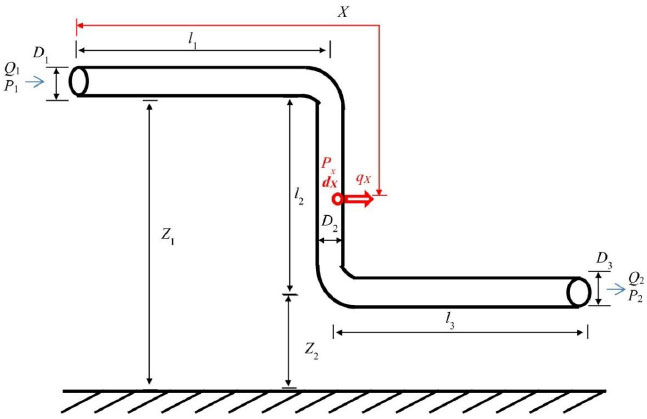
Case study.
The leak is located at a linear distance X from the inlet and occurs through a circular orifice of diameter dX. The flow rate of the leak qX (volume/time) is calculated by a discharge equation:
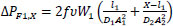
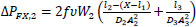
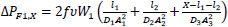
Where ρ is the density of the liquid, AX the cross-sectional area of the fracture, assuming a circular hole of diameter dX, PX and PATM are, respectively, the pressure inside the pipe at position X, and the atmospheric pressure. The valve constant K is set so that when dX and PX correspond, respectively, to a leak hole diameter equal to the largest pipe diameter in the network and to the highest pressure in the system, all inlet flow would be lost (qX equals Q1). The pressures at the point of the leak, PX, and the outlet P2 are calculated from the Bernoulli equations, where g is the gravitational acceleration constant.


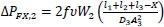
Where V1 and V2 are the linear velocities of the flow at the inlet and outlet of the pipe (V1=Q1/A1 and V2=Q2/A3, where A1 and A3 are respectively the cross-sectional areas of pipes of diameter D1 and D3 and Q2=Q1−qX), VX,1 and VX,2 are the linear velocities of the liquid, in the direction parallel to the pipe, just before and after the leak. Variables ΔPF1,X, and ΔPFX,2 are, respectively, the frictional pressure losses from the inlet to the leak position and from there to the outlet, and Z1, ZX, and Z2 are the vertical heights, with respect to a horizontal reference line, of the inlet stream, leak position, and outlet stream. The other terms of the equations depend on the leak position as shown below, where the mass flows W1 and W2 are calculated respectively as ρ×Q1 and ρ×Q2, υ is the specific volume of the fluid (1/ρ) and f is the friction factor.


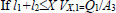
If l1+l2≤X

The lengths l1, l2, and l3, diameters D1, D2, and D3, and the average density ρ and viscosity of the liquid are known, as well as an estimate of the friction factor f. With the pressure P1 and the flow Q1, the Bernoulli equation allows the highest pressure of the system to be calculated, based on which the discharge constant K of Eq. (1) can be calculated. The unchanged system parameters were set to D1=D2=D3=5 cm, l1=l3=20 m, l2=10 m, Q1=10.65 m3/h, P1=2 atm, ρ=997 kg/m3 and f=0.0045.
3.2. A Priori Information
It is believed that the leak is equally likely to appear in any position and that its diameter is similarly expected to be anywhere between 1 and 5 cm. So, X is a uniformly distributed variable between 0 and 50 m, while dX is a uniform variable between 1 and 5 cm. While the literature reports specific probability distributions for pipe crack sizes across different materials, the uniform distribution is a “minimum information” distribution and may be used to reflect operators’ immediate knowledge once a leak is suspected. Simulating X and dX from their distributions and, using equations 1 to 18, the cumulative probability distribution of the outlet flow Q2 is calculated and shown in Fig. (2). Figs. 2 and 3 were produced by simulating 20’000 instances of X and dX from their probability distributions. The number of replications was found to be large enough that further increases did not noticeably change the cumulative probability distribution shape.
The cumulative probability distributions of Q2 conditional on whether the leak lies in the first (0<X<20), second (20<X<30), or third (30<X<50) pipe section are shown in Fig. (3). The section containing the leak alters the shape of the cumulative probability distribution of the outlet flow. Thus, observing the outlet flow should change the probability distribution of which section contains the leak. In the following, it is shown how an observation of Q2 can be used to update the initial beliefs about the possible leak location, and how this updated knowledge is used to decide how to search for the leak.
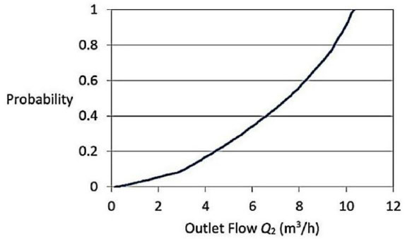
Marginal cumulative probability distribution of outlet flow.
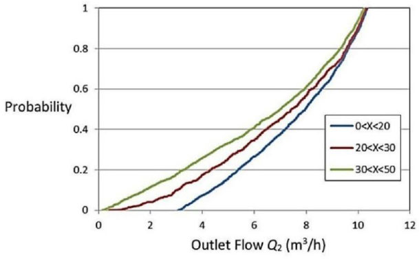
Cumulative probability distribution of outlet flow conditional on the leaking section.
3.3. Selection of the Section Review Sequence
Once it is noticed that the outlet flow decreases, indicating a leak, the pipe sections need to be checked to identify the section containing the leak. The system is divided into three sections:
(1) Section 1 (S1): the first horizontal section (with a length of 20m)
(2) Section 2 (S2): the central vertical section of 10m in length
(3) Section 3 (S3): the final 20 m pipe section.
The time needed to inspect sections 1, 2, and 3 is, respectively, Δt1, Δt2, and Δt3. When a leak is detected, a decision must be made regarding the order of inspection: which section to check first, which section to check next if no leak is found, and which section to inspect last if the leak remains undetected in the previously reviewed sections. The sequence of revisions is chosen through decision trees. Two cases are treated: an “a priori” case, in which the revision sequence is selected based on the initial beliefs on the leak location, and a “a posteriori” case, for which the a priori beliefs are updated using an observation of the outlet flow size, and the new knowledge state is used to choose the review sequence.
3.3.1. Recommended Review Sequence Based on A Priori Information
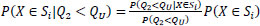
If no observations of the leak effects are made, the section review sequence is chosen based on a priori information, assuming that all points are equally prone to leaks, and the hole size can be anywhere between 1 and 5 cm. The checking of sections during the search for the leak is represented by the decision tree of (Fig. 4). Decision trees are read from left to right; boxes represent decisions, and circles represent uncertainties. The lines emanating from decisions stand for alternatives, while those emanating from uncertainties represent possible outcomes with their corresponding probabilities. The first decision is which section to inspect first, and the first uncertainty is whether the leak is found there. If the leak is not in the visited section, a decision is made on which section to visit next, which in turn leads to uncertainty about whether the leak is found in the newly visited section. The lines at the right end of the tree, which are not followed by any circle or square, are called tree tips, and the decision consequences are written next to them. Decision trees are solved from right to left by calculating the value of the uncertainties and decisions (called collectively nodes). The value of an uncertainty is the expected value of the set of nodes that are connected to its possibilities, while the value of a decision is the minimum value (as in this case, the problem aims to minimize the amount of lost liquid) among the set of nodes that are connected to its alternatives. The value of a decision situation is the value of the initial tree node. While there are several software packages in which decision trees can be implemented and solved, for this work, the relevant calculations were set up in MS Excel, using Macros explicitly programmed for the problem. The consequences are the result accrued by the decision maker for the alternatives and the outcomes leading to a specific tree tip. For example, if it is decided to inspect section 1 first (S1) and the leak is located here (X∈S1) the total volume of liquid lost is ∆t1E[qX|X∈S1], where E[qX|X∈S1] is the expected value of the leak flow rate if the leak is in Section 1. In this case, the consequences would be measured in cubic meters.
Since it was assumed that the leak has an equal probability of occurring at any point along the system, the probability that the break is in a section depends on the section length. The probabilities that the break is in one section, conditional on not being in another, are calculated by conditioning, e.g. P(X∈S2|X∉S1)=P(X∈S2∧ X∉S1)/P(X∉S1 )=P(X∈S2)/(1−P(X∈S1)). The probabilities and expected values of the leak flow rate conditional on the section in which the leak lies are presented in Table 1.
| P(X∈S1) | 0.4 | E[qX|X∈S1] | 3.21 |
| P(X∈S2) | 0.2 | E[qX|X∈S2] | 3.71 |
| P(X∈S3) | 0.4 | E[qX|X∈S3] | 4.30 |
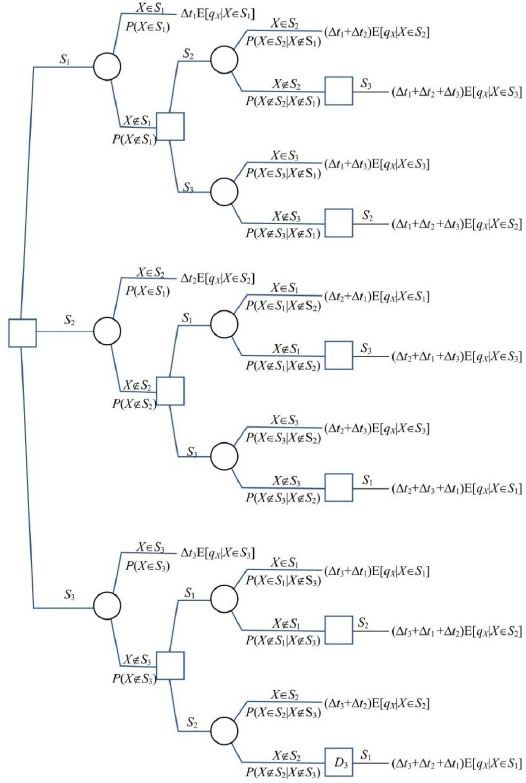
Decision tree based on a priori information.
By noting the wide range of outlet flow values resulting from a leak (Fig. 2), it can be concluded that the leak flow rate also shows significant variability. The decision, however, is based on the expected value of the leak flow rate, as it is assumed that the pipe owner has a linear preference for the volume of fluid lost (i.e., it is “risk neutral” regarding this quantity), in which case, the minimization of the expected value is an adequate decision objective. When the time to review each section is set as ∆t1 = ∆t2 = ∆t3 = 1 hour, solving the decision tree in Fig. (4) provides an optimal review sequence starting with Section 3, continuing with Section 1, and finishing with Section 2, corresponding to the expected amount of lost liquid of 6.4 m3.
3.3.2. Recommended Review Sequence Based on A Posteriori Information
A precise definition of a “rough observation of the size of the outlet flow” is provided by observing whether flow Q2 is bigger or smaller than a threshold value QU. This observation is used to update the a priori probabilities of which section is leaking, and the resulting a posteriori probabilities are used to select the section review sequence that minimizes the expected volume of liquid lost. The decision tree for this modification, shown in Figs. (5 and 6), starts with the uncertain event of observing a “large” (Q2≥QU) or “small” (Q2<QU) outlet flow. The tree substructures following the outcomes of this uncertainty are analogous to the tree based on a priori information, except that the probabilities and expected flow rates of lost liquid are conditioned by whether Q2 is small or large. The update of the probabilities is done through Bayes’ theorem.
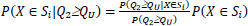
P(Q2<QU) can be calculated from the marginal distribution of Q2. As an example, let QU equals 3.2 m3/h and the event Q2<QU, which has a marginal probability of P(Q2<QU)=0.1 (Fig. 2) and a probability conditional on the leak being in Section 1 of P(Q2<QU|X∈S1)=0.005 (Fig. 3). Based on its length, the a priori probability of Section 1 leaking is P(X∈S1)=0.4, so the corresponding a posteriori probability given Q2<QU is P(X∈S1|Q2<QU)=P(Q2<QU|X∈S1)×P(X∈S1)/P(Q2<QU)=0.005×0.4/0.1=0.02. This means that if the outlet flow is smaller than 3.2 m3/h, it is extremely unlikely that the leak lies in Section 1.
Top section of the decision tree based on a posteriori information.
Bottom section of the decision tree based on a posteriori information.
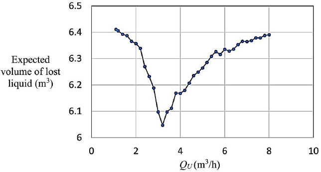
The threshold value QU should be selected so that the expected amount of lost liquid (i.e., the value calculated by solving the tree) is minimized. If ∆t1, ∆t2, and ∆t3 are set to one hour, (Fig. 7) shows that QU should be set to 3.2 m3/h to reduce the expected amount of fluid lost.
For QU=3.2 m3/h, the conditional probabilities of the leak being in each section and expected flow rates of lost fluid are shown in Tables 2 and 3. The calculated probabilities of the outlet flow being bigger or smaller than QU are, respectively, P(Q2≥3.2)=0.90 and P(Q2<3.2)= 0.10.
| P(X∈S1| Q2≥3.2) | 0.44 | E[qX|X∈S1,Q2≥3.2] | 3.08 |
| P(X∈S2| Q2≥3.2) | 0.20 | E[qX|X∈S2,Q2≥3.2] | 3.11 |
| P(X∈S3| Q2≥3.2) | 0.36 | E[qX|X∈S3,Q2≥3.2] | 3.17 |
Expected value of the amount of liquid lost.
| P(X∈S1|Q2<3.2) | 0.02 | E[qX|X∈S1,Q2<3.2] | 6.58 |
| P(X∈S2|Q2<3.2) | 0.22 | E[qX|X∈S2,Q2<3.2] | 7.37 |
| P(X∈S3|Q2<3.2) | 0.76 | E[qX|X∈S3,Q2<3.2] | 7.94 |
| Decision based on information | Recommended section review sequence | Expected volume of liquid lost (VT) in m3 | ||
|---|---|---|---|---|
| A priori | S3→S1→S2 | 6.43 | ||
| A posteriori | Large outlet flow (Q2≥3.2) | S1→S3→S2 | 5.49 | 6.03 |
| Small outlet flow (Q2<3.2) | S3→S2→S1 | 10.90 | ||
If the time needed to check the sections is taken as ∆t1 = ∆t2 = ∆t3 = 1 hour, Table 4 presents the recommended review sequences with a priori information, and the recommended ones based on a posteriori information for the cases when (Q2≥3.2) and (Q2<3.2). The notation Si→Sj→Sk is used to represent a review sequence beginning in Section i, continuing with Section j, and finishing with Section k.
Let VT, APR be the expected amount of lost liquid when the recommended sequence is based on a priori information, and VT, POS be the corresponding value when the sequence is chosen based on updated information. In the table VT, APR = 6.43 m3 and VT, POS = 6.03 m3. The advantage of observing Q2 in choosing the review sequence, instead of relying solely on prior knowledge, is denoted as ∆VT and calculated by VT, PR −VT, POS. From the table, ∆VT is 0.40 m3. ∆VT is called “observation value”.
3.3.4. Effect of Section Inspection Times
To analyze the effect of the section inspection times on the recommended sections review sequence, ∆t1 was set to one, while the ratios ∆t3/∆t1 and ∆t2/∆t1 were varied. For each case, the decision trees of (Figs. 4-6) were solved to determine the recommended inspection order.
3.3.4.1. Inspection Sequences Based on a Priori Information
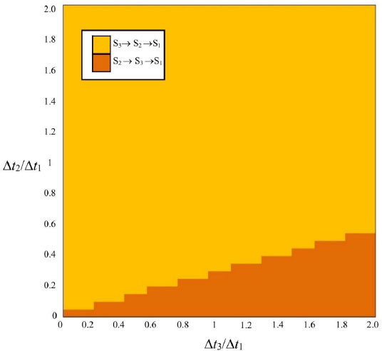
The recommended sequences of visits are shown chromatically in Fig. (8), for the case in which only a priori knowledge is used. If the time it takes to check Section 1 is small relative to that of the other sections (large values of ∆t3/∆t1 and ∆t2/∆t1, near the top right corner of (Fig. 8), Section 1 should be checked first. Similarly, if Section 2 can be checked quickly than the other sections (near the bottom right corner), this section is reviewed first. Generally, if the time to review a given section is considerably shorter than the other sections, the model recommends checking that section first. This is because if the leak is there, it can be stopped promptly, and if it is not, little time has been invested. The area of the graph for which the model recommends visiting Section 2 first is smaller than the corresponding areas for which the first-visited section is either Section 1 or Section 3, as Section 2 is the shortest and thus the least likely to harbor the leak. Moreover, among the sequences starting with either Section 1 or 3, those reviewing Section 2 next are restricted to a smaller figure area than those checking Section 2 last.
On the other hand, the area of (Fig. 8) where it is recommended to start reviewing Section 3 is larger than the corresponding area recommending starting in Section 1, even though the two sections have the same size and, therefore, the same a priori probability of leaking. This is because leaks in Section 3 tend to have higher flow rates than those in Section 1, so they must be addressed earlier.
3.3.4.2. Inspection Sequences Based on A Posteriori Information
The case in which the observation of the outlet flow being bigger or smaller than a threshold value QU is used to update the a priori information is treated next. QU is selected to minimize the expected value of the total liquid lost, and may differ depending on the values of ∆t2/∆t1 and ∆t3/∆t1. However, (Fig. 9) shows that the minimizing QU value remains approximately equal to 3.2 m3/h for the range of ∆t2/∆t1 and ∆t3/∆t1 values of interest.
Recommended review sequences based on a priori information.
Expected value of the amount of liquid lost for different values of ∆t2/∆t1 and ∆t3/∆t1.
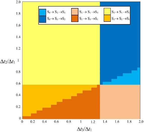
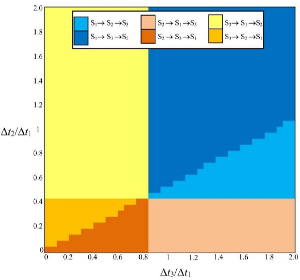
The recommended inspection sequences for large outflows (Q2(QU), indicating a small leak) are shown in Fig. (10). Since a small leak is more likely to be in Section 1, this is the section to be visited first for most of the (∆t2/∆t1, ∆t3/∆t1) space, save for the case in which the review time of the other sections is sufficiently low relative to that of Section 1, specifically if ∆t2/∆t1<0.45 or ∆t3/∆t1<0.85. This condition is more restrictive for sequences that begin with Section 2, as the leak is less likely to occur in this section.
If the outflow is less than QU, indicating a significant leak, the recommended inspection sequences, as ∆t2/∆t1 and ∆t3/∆t1, are varied and shown in Fig. (11). In this case, the probability that the leak is in Section 3 is higher, so Section 3 is reviewed first in most cases, except when ∆t2 is small and ∆t3 is large, in which case Section 2 is reviewed first. Although the a priori probability of the leak being in Section 1 is twice that of Section 2, if the leak is large, it is very unlikely to be in Section 1, so Section 2 is the last to be checked.
Recommended review sequences based on a posteriori information given Q2≥3.2.
Recommended review sequences based on a posteriori information given Q2<3.2.
The difference between the expected value of lost liquid when the inspection sequence is decided with a posteriori information and the corresponding quantity using a priori information is called “observation value” and provides a measurement of the worth of the measurement used for updating the a priori information. This quantity is shown in Fig. (12). When the observation value is null, it means that the recommended inspection sequence is the same for the a priori decision and for both instances of the a posteriori one. If Section 3 can be reviewed swiftly (low value of ∆t3), the observation value is small, as the a priori and a posteriori inspection sequence selections recommend reviewing this section first, given that the most significant leaks are expected to be in here. The important values of the observation value are associated with cases in which reviewing Section 3 would take a lot of time (big value of ∆t3), as in this case, the solution of the decision problem with a posteriori information changes the recommended sequence depending on the observed outlet flow.
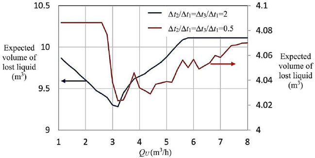
Figure 13 shows a plot of the observation value when ∆t2/∆t1 is fixed to one and ∆t3/∆t1 is varied. Below this plot, color bars indicate the inspection sequence recommended for the ∆t3/∆t1 value directly above on the horizontal axis, the top bar stand for decisions based on a priori information, while the middle and bottom horizontal bars show, respectively, the sequence based on a posteriori information, for the cases of a big (Q2>QU) or small (Q2≤QU) outlet flow. For example, for ∆t3/∆t1 below approximately 0.82, all recommended sequences start reviewing Section 3, with the recommended sequence based on a posteriori information if the outlet flow is small, selecting Section 2 to be visited next.
4. DISCUSSION
Decision Analysis, as a discipline, emphasizes the importance of making the most of the available information when choosing a course of action. Such a situation occurs when a leak occurs in a hydraulic distribution system composed of several connected sections, and a section-review sequence should be chosen to locate the leak, minimizing the expected loss of liquid. In all situations, at the very least, two pieces of information are available. First, not all the sections are equally likely to harbor the leak, as longer sections are more likely to leak than shorter ones, if it is believed that all points along the pipe have the same probability of presenting a crack. Second, sections composed of pipes of larger diameter and under higher liquid pressure are more likely to exhibit leaks at higher flow rates than sections composed of smaller-diameter pipes under lower pressure. Additionally, the selection of the review sequence should consider the time needed to review each section. If a long time is invested in visiting a section that fails to harbor the leak, more liquid will be lost.
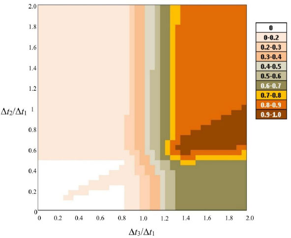
Observation value (in m3) given ∆t2/∆t1 and ∆t3/∆t1.
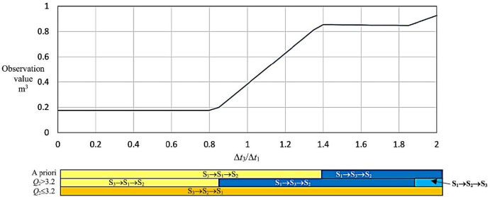
Observation value and recommended sequences for fixed ∆t2/∆t1 =1.
This work has shown how the above information can be coded as probability distributions and, when complemented with a rough hydraulic model, used to decide the sequence of inspections in a three-section pipe system. The probabilities and flow information produced by simulation are fed into decision trees that select the recommended section review sequence. Two cases are compared, when the sequence is chosen based on a priori information (e.g., the belief that the probability of a leak appearing in a section is proportional to the section length) and when the sequence selection is based on a “a posteriori” information state, in which the a priori is information is updated in a Bayesian scheme, using the observation of whether the flow reaching the end of the system is above or below a threshold value. This threshold value is optimized to minimize the expected amount of lost liquid.
CONCLUSION
In contrast to previously reported research, this work shows how a Decision Analytic perspective can be used to take advantage of the available knowledge and modelling tools, no matter how scarce the former or basic the latter, to improve the search for leaks in a multi-section hydraulic system, considering the time needed to review each section. The presented approach also has the advantage of using a basic hydraulic model, so it´s much simpler than other reported leak location algorithms that are too complex to find general application or to be applied quickly by hydraulic engineers without advanced mathematical training.
One of the shortcomings of decision trees is that they grow exponentially as more alternatives are added to the problem. In such a case, the problem can be represented using influence diagrams, which maintain the problem's decision structure without drawing trees. Influence diagrams, though, still need to solve the same combinatorial problem as decision trees. In cases where this latter approach becomes computationally burdensome (e.g., problems with a very high number of alternatives and outcomes), approaches such as partial tree search have been proposed to provide a solution.
AUTHORS’ CONTRIBUTIONS
The authors confirm their contribution to the paper as follows: M.L.C.: Study conception and design; G.J.E., V.V.R.: Draft manuscript. All authors reviewed the results and approved the final version of the manuscript.
AVAILABILITY OF DATA AND MATERIALS
All the data and supporting information are provided within the article.
ACKNOWLEDGEMENTS
Declared none.