All published articles of this journal are available on ScienceDirect.

Modeling and Simulation of Pressure Equalization Step Between a Packed Bed and an Empty Tank in Pressure Swing Adsorption Cycles
Authors Info & Affiliations
Abstract
Background:
It is of paramount importance to pay a great attention when modeling pressure equalization step of pressure swing adsorption cycles for its notable effect on the accurate prediction of the whole cycle performances. Studies devoted to pressure equalization between an adsorption bed and a tank have been lacking in the literature. Many factors could affect the accuracy of the dynamic simulation of pressure equalization between a bed and an empty tank.
Methods:
The method used for the equilibrium pressure evaluation has a significant impact on simulation results. The exact equilibrium pressure (Peq) obtained when connecting an adsorption column and an empty tank could only be obtained by numerical simulation given the complexity of the set of partial differential equations.
Results:
It has been shown that, with some simplifying assumptions, one can analytically determine Peq with satisfactory precision. The analytical solution proposed permits to assess rapidly the equilibrium pressure and the equilibrium mole fraction of the adsorbable species in the tank (Yeq) and without the need to resort to a cubersome modeling.
Conclusion:
Based on the comparisons presented, one can conclude that the agreement between the experimental and numerical results relative to Peq and Yeq is very satisfactory.
1. INTRODUCTION
The modeling of varying pressure steps of pressure swing adsorption cycles have received a great deal of attention because of the great effect of these steps on the accurate prediction of whole cycle performances. These steps comprise pressurization, blowdown and equalization. However, until recently, the main attention has been given to pres- surization and depressurization. The incorporation of a pressure equalization step has been proposed for the first time by Berlin in 1966 [1]. The pressure equalization step has two purposes: To save the mechanical energy contained in the gas of a high pressure bed, and to recover a part of the product that would otherwise be lost in the blowdown. One of the ways to do this is to use the high-pressure gas removed during the cocurrent depressurization step to repressurize other adsorber by pressure equalizations. It is done by connecting the ends of two beds at a particular stage of the cycle. Thus, pressure equalization steps enable gas separations to be realized economically on a large scale.
Very few articles entirely devoted to the study of the equalization step of PSA cycles have been published. Apart from some adsorption simulators, capble of simulating the step with no simplifying assumptions such as ASPEN Adsorption, the equalization step has been generally treated as an ordinary depressurization for the high pressure bed (from PH to Peq ) and as an ordinary pressurization for the low pressure bed (from PL to Peq ) with a constant pressure at the open end of the bed (Peq ). The equilibrium pressure Peq reached at the end of the equalization step is evaluated after considering simplifying assumptions and rough approximations [2-5]. In many approaches, the pressure history during equalization is assumed to follow some simple law, e.g. exponential or linear, similarly to the conventional depressurization or pressurization steps.
Warmuzinski [6] has developed a simple analytical formula to measure energy savings resulting from the pressure equalization step. Warmuzinski and Tanczyki [7], have also proposed a formula for calculating the equilibrium pressure Peq in the case of linear uncoupled isotherms and no breakthrough of the more strongly adsorbed component from the bed undergoing depressurization. Delgado and Rodrigues [8] have analyzed the effect of three types of boundary conditions on the time and spatial profiles of the pressure equalization step of a Skarstrom PSA cycle. Chahbani and Tondeur [9] have simulated the dynamics of the pressure equalization step and evaluated the equilibrium pressure numerically and analytically.They have shown that in some simple cases only the pressure equalization step can be decomposed into independent pressurization and depressurization steps and that the constant pressure at the open end of the pressurized or depressurized bed should be accurately estimated prior to this decomposition. Yavary et al. [11] have found that the analytical solution, proposed by Chahbani and Tondeur for the evaluation of the equilibrium pressure, provides a more realistic mathematical procedure with respect to the use of an arithmetic mean for the calculation of the final pressure for the pressure equalization steps. Yavary et al. [12] have also shown that the number of pressure equalization steps affects significantly both purity and recovery of product. Therefore, the number of pressure equalization steps must be considered as an important process parameter in evaluating process performance.
In 1964, prior to Berlin’s improvement of the Skarstrom cycle, Marsh et al. [10] have suggested another idea for reducing blowdown loss. Besides the two adsorption beds, an empty tank is used. At the end of the high-pressure adsorption step but well before breakthrough, the feed flow is stopped and the product end of the high-pressure bed is connected to the empty tank where a portion of the compressed gas, rich in the product, is stored. The blowdown of the high-pressure bed is completed by venting to the atmosphere in the reverse-flow direction. The stored gas is then used to purge the bed after which the bed is finally purged with product gas. The product comsumption during purge is reduced, thereby increasing the recovery. Tondeur and Wankat [13] have described a number of PSA cycles that implement empty tanks, and have shown that the sequences in complex multi-column, multi-step cycles can be emulated by a system comprising a single column and a multiplicity of empty tanks. It is therefore of general interest to revisit the pressure equalization between a column and an empty tank.
In the work previously cited, we have studied in detail pressure equalization between two packed columns. In this work, we will try to extend the previous study to pressure equalization between a column and a tank in the sense that studies devoted to pressure equalization with a tank have been lacking in the literature.
2. MODELING
The simulation of a fixed-bed adsorber requires the numerical solution of the governing partial differential equations: mass, heat and momentum balances as well as mass transfer kinetics.
2.1. Mass Balance for the Packed Bed
A differential fluid phase mass balance for the component i is given by the following axially dispersed plug flow equation:
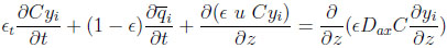 |
(1) |
with ϵt = ϵ + (1 − ϵ) ϵp, being the total porosity.
The overall mass balance for the bulk gas is given by:
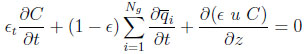 |
(2) |
wherein u is the interstitial fluid velocity, ϵ the bed or the interparticle void fraction,ϵp the intraparticle void fraction or porosity,  the total bulk phase concentration, Z being the compressibility factor of the gas mixture.
2.2. Heat Balance for the Packed Bed
A heat balance for the bed can be written as:
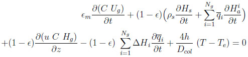 |
(3) |
with
 |
For completeness, this equation accounts for heat transfer between the column and some environment at a temperature Te. However, in the numerical application, only the adiabatic case will be considered. In the following, the heat capacities of adsorbed species (cpia ) are supposed to be equal to those in gas phase (cpig ).
2.3. Momentum Balance
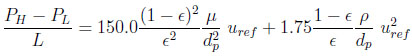
Ergun’s law is used to estimate locally the bed pressure drop.
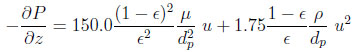 |
(4) |
where µ is the gas mixture viscosity, ρ the gas density and dp the particle diameter.
2.4. Mass Balance for the Empty Tank
A fluid phase mass balance for the component i in the tank is given by the following equation:
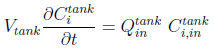 |
(5) |
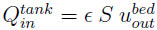 is the volume flowrate at the tank inlet which is equal to the volume flowrate at the bed exit,
  is the gas velocity at the bed outlet.
  and
and  are the concentrations of gas component i at the tank inlet and in the tank respectively. The tank is considered perfectly mixed.
2.5. Heat Balance for the Empty Tank
A heat balance for the tank can be written as:
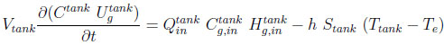 |
(6) |
with  ,the gas concentration and the gas internal energy in the tank,
  and
and  the gas concentration and the gas enthalppy at the tank inlet, Stank the heat transfer surface of the tank.
2.6. Numerical Method
The foregoing models require the simultaneous solution of a set of partial differential and algebraic equations (overall and component mass balance equations, heat balance equation and momentum balance equation). The above equations are easily rewritten using dimensionless variables, (P/Pref , u/uref ,T /Tref, ............). The well-mixed cells method is used to discretize the system. The resulting system of ordinary differential and algebraic equations are solved by the DDASSL integration algorithm of Petzold [14] DASSL is designed for the numerical solution of implicit systems of differential/algebraic equa-tions written in the form F(t,y,y’)=0, where F, y, and y’ are vectors, and initial values for y and y’ are given. The time derivatives are approximated by the Gear formula BDF (Backward Differentiation Formula) and the resulting nonlinear system at each time-step is solved by Newton’s method. The full description of the code can be found in reference [14]. The runtime of the code is less than one minute for an ordinary computer equipped with Intel Core 2 Duo Processor E4700 (2M Cache, 2.60 GHz, 800 MHz FSB).
2.7. Boundary and Initial Conditions
As shown in Fig. (1), the boundary conditions are as follows:
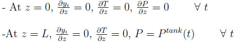 |
The whole step can be considered as a depressurization of the bed and a pressurization of the tank. The pressure at the outlet of the bed or at the inlet of the tank varies with time.
The initial conditions for the bed and the tank should also be defined. The pressure is PH in the bed and PL in the tank. The axial profiles of composition and temperature at t = 0 in the bed correspond to those of the final state attained during the step preceding the equalization step.
The effluent of the column is the feed of the tank. Thus, pressure, temperature and composition at the outlet of the bed are identical to those prevailing at the inlet of the tank.
This paper will only focus on the assessment of the equilibrium pressure obtained when connecting an adsorption column and a tank and will not deal with energy consumption optimization and product recovery. In fact, one of the goals of the equalization step is to collect the portion of product-rich gas ahead of the concentration wave (in the mass transfer zone). The amount of gases transferred to the tank strongly depends on the initial location of the concentration wave. In a real situation, the optimized tank volume is related to the initial location of the concentration wave front in the bed. The best situation would be that the adsorbable species is just about to breakthrough when the pressure is equalized. The packed bed is initially uniformly loaded. The reason of starting the simulation from a uniformly loaded bed is that it would be easy, as we shall see later when the bed is initially uniformly loaded, to validate the experiments carried out without having to worry about the precise position of the front in the column before the pressure equalization step. The validation is simply done through the comparison of the values of the equilibrium pressure and the molar fraction of the adsorbable gas in the tank at the end of the step obtained numerically and experimentally.
In practical operations, the column and the tank are separated by valves and tubings, which could in principle be included in the modeling. The work presented herein considers that the pressure drop through the valves and tubings is negligible. This does not affect the value of equilibrium pressure attained at the end of the step, it does only modify the dynamics of the pressure equalization. in fact, the presence of significant pressure drop tends to increase the duration of the step.
When flow goes through a valve or any other restricting device, it loses some energy. The flow coefficient (cv ) is a designing factor which relates pressure drop (∆P) across the valve with the flow rate (Q). Each valve has its own flow coefficient. This depends on how the valve has been designed to let the flow going through the valve. Therefore, the main differences between different flow coefficients come from the type of valve, and of course the opening position of the valve. At same flow rate, higher flow coefficient means lower drop pressure across the valve. Depending of manufacturer and type of valve, the flow coefficient can be expressed in several ways.
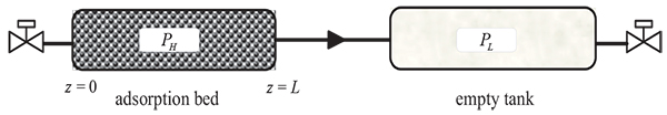
Simulating of varying pressure steps without the incorporation of a valve equation shows a notable disparity with experimental results as can be seen in Fig. (2) for depressurization. This is why it is indispensible to take into account the significant pressure drop across the valve in the modeling. The two following valve models could be used:
 [
[avec
- C concentration (mol/m3)
- Q molar flow rate (mol.s−1)
- ∆P pressure drop across the valve (Pa)
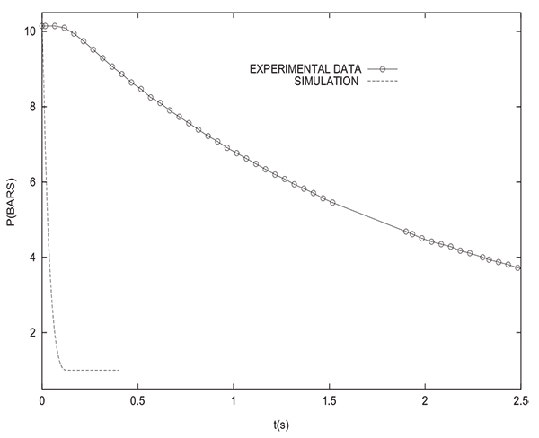
Figs. (3 and 4) show that the incorporation of a valve equation in the modeling permits to obtain a good agreement between experimental results and simulations. The values of the flow coefficients given by the two models are different. However, it must be noted that the values of flow coefficients obtained herein are only valid for the experimental PSA setup studied and they can not be used for simulating different theoretical PSA systems.
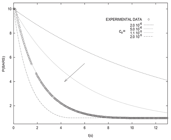
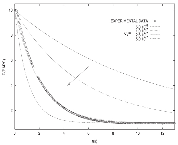
However, it should be mentioned that, in the following, a valve equation will be only used when comparing simulation and experimental results. As previously mentioned, the assessed equilibrium pressure is not affected by the presence or absence of a valve equation in the modeling.
2.8. Analytical Solution for the Equilibrium Pressure
As presented above, the model can not be analytically solved. However, if the following simplifying assumptions are considered, an analytical solution can be obtained. For the purpose of comparison, we shall examine the results of this analytical approximation as well as the full numerical solutions:
- The process is isothermal
- The column and the tank are considered homogeneous at the initial and final states.
- The gaseous and solid phases are in equilibrium at the initial and final states.
- The equalization time is large.
The fourth condition implies that the column and the tank become identical at the end of the equalization step. This approximation may appear very rough, but as will be seen later, the value of the equalization pressure obtained considering these hypotheses is more accurate than the arithmetic or geometric mean.
For the sake of simplicity, the resolution is restricted to the case of a gas mixture composed of two species, one of which is inert (I) whereas the other is adsorbable (A).
The total number of moles in each bed at the initial state are
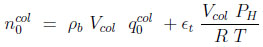 |
(7) |
and
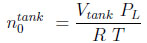 |
(8) |
Where ϵt is the total porosity (ϵ + (1 − ϵ)ϵp). The first term on the right hand side represents the moles adsorbed. In equations (7) and (8), the subscript 0 refers to the initial state.
The constitutive equations of the model are written as follows:
-Conservation of the total number of moles in the the column
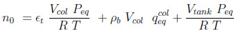 |
(9) |
Where the total number of moles in the system n0 is given by the sum of Equations (7) and (8). The subscript eq refers to the end of the equalization step.
-Conservation of the total number of moles of inert component I
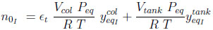 |
(10) |
-Langmuir adsorption equilibrium in column 1 after equalization
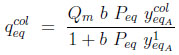 |
(11) |
-Summation of mole fractions in the column
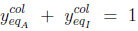 |
(12) |
-Summation of mole fractions in the tank
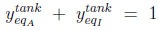 |
(13) |
The system of 5 equations (9) to (13) relates 6 unknowns (the four mole fractions y, the adsorbed quantity qcoleq and Peq ). By substituting equations (11) to (13) into Equations (9) and (10), three of these variables can be eliminated, leaving a system of two equations with three unknowns, Peq , ycoleqI and ytankeqI for example. To resolve analytically, an additional assumption needs to be made. We shall assume here that the column and the tank have identical gas phase compositions at the end of equilibration (thus, ycoleqI = ytankeqI ), leaving only two unknowns. The analytical resolution then leads to a quadratic equation whose positive root is
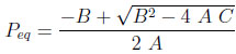 |
(14) |
with
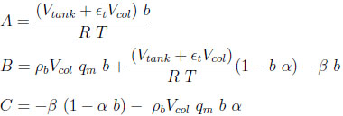 |
where
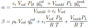 |
The inert species molar fraction is:
 |
(15) |
The adsorbable species molar fraction is
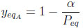 |
(16) |
In the case of more than one adsorbable species, a similar set of conservation and equilibrium equations may be written, and with the assumption of equal gas-phase compositions of the columns and the tank in the end state, this set determines the end pressure Peq. However, a compact analytical solution is probably impossible, and the solution for Peq has to be found numerically.
In the case where the column and the tank initially contain only one species (adsorbable or inert), one can easily obtain the following formula for the equilibrium pressure
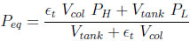 |
(17) |
If the column and the tank have the same volume Peq becomes:
 |
(18) |
3. RESULTS AND DISCUSSION
The numerical simulations presented herein concern methane uptake from hydrogen by using activated carbon. H2 is supposed to be a non-adsorbed species. The adsorption equilibrium isotherm of CH4 on activated carbon is given by the Langmuir model
 |
(19) |
The parameters Qm and b are function of temperature:
 |
(20) |
 |
(21) |
Table 1 gives the values of ki parameters and adsorption heat used in simulations.
| Langmuir parameters | |
|---|---|
| k1 | 7.063 103 mol/m3 |
| k2 | 13.610 mol/(m3K) |
| k3 | 3.07110−8 1/Pa |
| k4 | 1574.1 K |
| Adsorption heat (∆H) | 20.0 kJ/mol |
The model requires the assessment of the physical properties of the gas mixture. The compressibility factor is calculated following the method of Lee-Keesler [17]. The viscosity of each pure gas is estimated by Lucas method [17] whereas the viscosity of the mixture is evaluated by the Reichenberg method [17]. The compressibility factor (Z), the mixture viscosity (µ) as well as the gas density (ρ) vary with temperature, pressure and composition, therefore they are calculated at every computation step.
The adsorbent physical properties are given in Table 2. The heat capacities of the various gases are calculated by using an equation of the following form:
 |
(22) |
| Apparent density (ρp) | 830 kg/m3 |
| Intraparticle porosity (ϵp) | 0.6 |
| Particule diameter (dp) | |
| 0.1 10−3 m |
The constants a, b, c and d for the two gases are listed in Table 3.
| a | b | c | d | |
|---|---|---|---|---|
| H2 | 27.14 | 9.274 10-3 | ||
| -1.381 10-5 | 7.645 10-8 | CH4 | 19.25 | 5.213 10-2 |
Table 4 gives the operating conditions used for computations. All the following simulations are in the adiabatic case (h=0).
| Initial pressure (P0) | |
|---|---|
| Bed | 5.0 105 Pa |
| Tank | 1.0 105 Pa |
| Initial temperature | 298 K |
| Initial CH4 mole fraction | |
| In the bed | 0.5 |
| In the tank | 0.0 (pure hydrogen) |
| Bed length (L) | 2.0 m |
| Interparticle porosity (ϵ) | 0.4 |
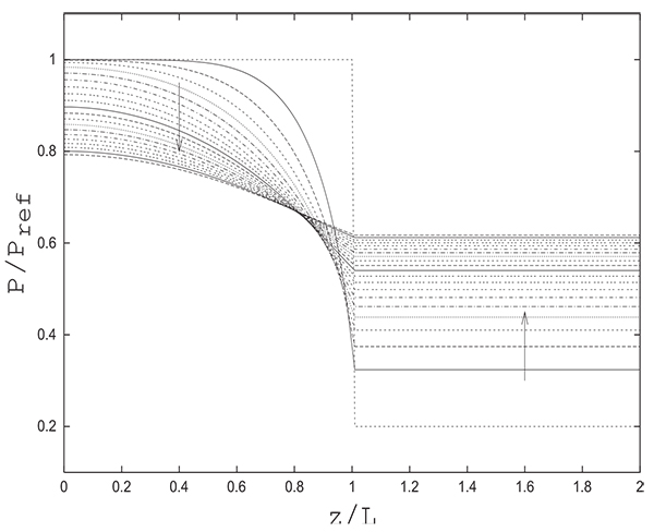
In what follows, we will consider a fully saturated column at a high pressure PH and a tank at a low pressure PL containing only inert (pure product). The volume of the tank is equal to that of the column. Fig. (5) gives the evolution of the pressure in the column and the tank during time. The pressure in the tank, as mentioned previously, is uniform. X-coordinates (z/L) varying from 0.0 to 1.0 correspond to the column, and x-coordinates from 1.0 to 2.0 are relative to the tank. This does not mean that the tank has the same length as the column.This representation is chosen to show both the pressure variation in the column and the tank, since the numerical solution gives only a single pressure value in the tank and not a longitudinal profile.
The reference pressure is taken as Pref = PH . The reference velocity uref is calculated using Ergun’s correlation as follows:
 |
(23) |
The pressure in the tank is uniform and is nearly equal to that prevailing at the column exit.
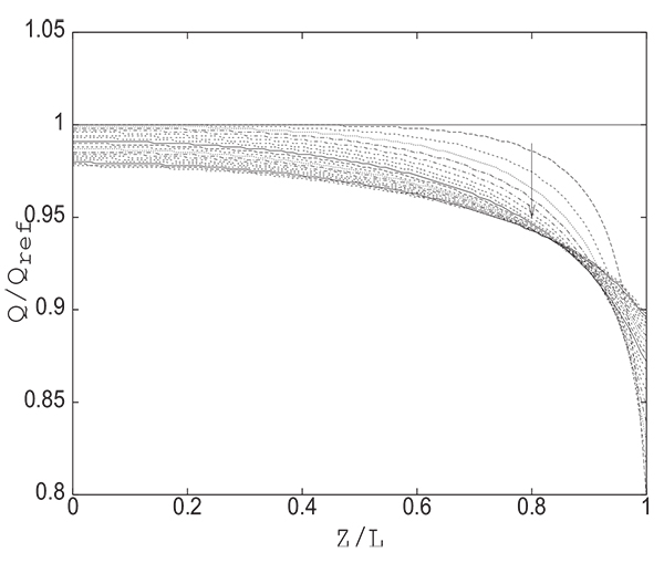
Fig. (6) shows the change with time of axial velocity profile for the column. These profiles are similar to those obtained in the cases of depressurization of a column and pressure equalization between two columns (Chahbani and Tondeur, 2010).
Given that the pressure at the open end of the column is variable in time, it would not be judicious to treat pressure equalization step just as a simple depressurization step with a constant pressure Peq at the open end of the column even if one succeeds to accurately estimate Peq as previously mentioned. This procedure was successfully done for pressure equalization between two packed beds in some cases (Chahbani and Tondeur, 2010), thus allowing substantial savings in computational time besides the simplification of modeling.
Consequently, for pressure equalization between a bed and an empty tank, the whole step could not be decomposed into two independent steps, namely depressurization of the bed and pressurization of the tank with a constant pressure at the open end (Peq ). When connecting together a bed and an empty tank having different initial pressures, it is expected to get always a varying pressure at the junction point.
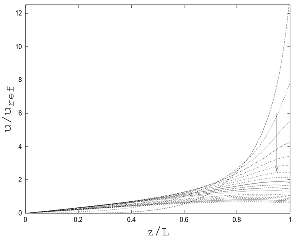
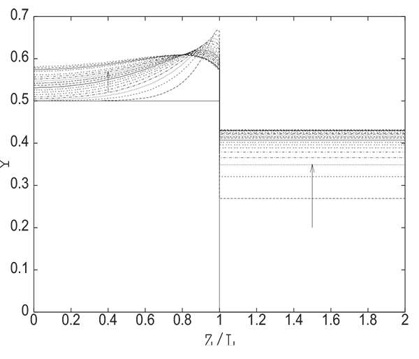
Fig. (7) gives the evolution of the adsorbable species molar fraction along the bed and in the tank during equalization. One can note that in the vicinity of the open end of the column, the adsorbed quantity q decreases drastically just after the beginning of the operation and then begins to increase gradually as shown in Fig. (8). This explains clearly the evolution of the adsorbable species molar fraction near the open end of the bed. In fact, it increases at the beginning of the equalization step due to desorption as the pressure diminishes notably at the open end of the column. The adsorbable species molar fraction then decreases regularly as the pressure starts to increase continuously tending towards the equilibrium pressure Peq . After the phase of desorption, occuring during the first moments of the pressure equalization in the vicinity of the open end of the column, an adsorption phase follows due to the increase of the partial pressure of the adsorbable gas.
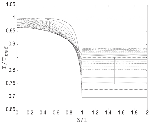
The substantial reduction of pressure at the open end of the column at the beginning of the pressure equalization step inevitably leads to an increase in desorption. This results in a temperature decrease as can be seen from Fig. (9) giving the change with time of axial profiles of temperature in the bed and in the tank. The pressures at the open end of the column and in the tank evolve simultaneously from 1 bar to Peq. The pressure in the tank continuously increases from 1 bar to Peq while at the open end of the column it drops rapidly from 10 bar (initial value of pressure in the column) to 1 bar (initial value of pressure in thank) and then begins to increase as the pressure in the tank increases. Inside the column, the decrease of temperature is continuous due to continuous desorption caused by the decrease of pressure. The temperature increase at the open end of the column which follows a temperature decrease observed at the beginning of the step is of course due to the adsorption (see Fig. 8) caused by the increase in pressure as can be seen in (Fig. 5).
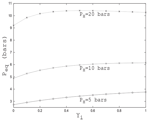
The equilibrium pressure Peq is not sensitive to the initial state of the column as is the case of pressure equalization between two columns. From Fig. (10), giving Peq variation in function of the initial adsorbable species molar fraction in the column for several values of PH , one can see that for a given initial pressure PH , the difference between Peq values for all initial states is of the order of 1 bar. In addition, the equilibrium pressure is not affected by the initial state of the tank. In fact, the value of Peq obtained is the same whether the tank is filled with inert or adsorbable gas. This can be explained by the fact that the phenomenon of adsorption does not intervene in the tank.
It is clear that, given the complexity of the set of partial differential equations, it is very difficult to analytically determine with satisfactory precision the final pressure Peq attained and it therefore seems necessary to resort to numerical simulation to get reliable results. A reliable value of Peq is of paramount importance when assessing pressure swing adsorption cycles performances. Peq is usually calculated by a trial and error procedure. A reasonably good initial guess of Peq can speed up notably the whole procedure.
Fig. (11) shows a comparison between the variations of Peq with Yi obtained by numerical simulation and analytical solution proposed herein for PH = 20 bars .
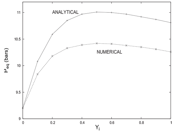
It is interesting to note that both solutions provide the same trend of evolution of Peq with Yi. In both cases, the equilibrium pressure increases initially with Yi to attain a maximum value and then begins a slight decrease. The difference between the two solutions does not exceed 0.5 bar despite the rough approximations considered for the analytical solution. The value of Peq given by the analytical solution is always greater than the one given by the numerical solution. For Yi = 0 (the column contains only an inert gas), note the coincidence of the numerical value of Peq with that obtained analytically (from equations 17 or 18). One can often resort to comparison between numerical and analytical solutions in special cases to prove the reliability of modelling and numerical resolution. It is the case herein.
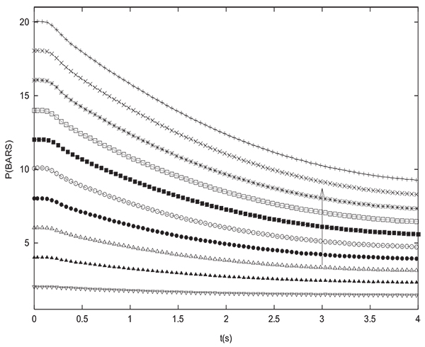
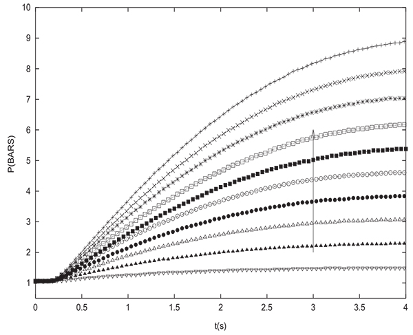
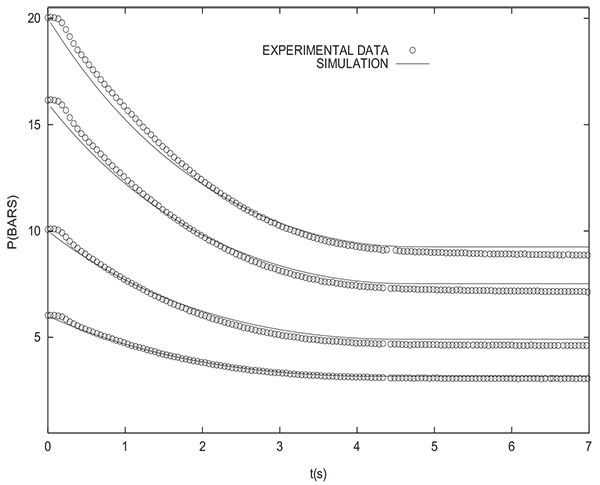
To validate the simulation results, many pressure equalization experiments have been carried out and compared to simulations. Figs. (12 and 13) show the experimental variation with time of pressure at the closed end of the column and inside the tank during equalization respectively for many different initial values of PH (between 2 and 20 bars with an increment of 2 bars). The initial pressure prevailing in the tank is always PL=1 bar. The column and the tank contain initially pure hydrogen. For the latter experiments, the tank is an empty column having the same length and diameter as the packed one (D=0.05 m, L=1 m). The arrow indicates direction of increasing initial PH value. Pressure at the closed end of the bed decreases while the pressure in the tank increases during equalization until reaching the equilibrium pressure. For the different experiements, the value of Peq obtained is very close to the one given by the equation (17) which is valid for a non adsorbable gas. Fig. (14) gives a comparison between time change of pressure at the closed end of the column obtained both experimentally and numerically. It can be seen that the simulation allows to model the experimental results in a satisfactory way. The slight difference that can be noticed is due to the fact that the volume of tubings relating the column and the tank is not taken into account in modeling. This is why the value of equilibrium pressure obtained by simulation is slightly greater than the experimental one. The same remarks are valid for time variation of pressure in the tank.
Let us now compare numerical and experimental results when the packed bed initially contains a binary gas, one of which is adsorbable (methane). Fig. (15) shows the experimental change with time of pressure at the closed end of the column and inside the tank during equalization for many initial states of the column. In fact, prior to pressure equalization, the column is in equilibrium with different binary mixtures of H2 and CH4 (for yCH4 =0,0.1, 0.2 and 1.0) at PH =10 bars whereas the tank is filled with H2 at PL=1 bar.
The arrow indicates direction of increasing initial methane molar fraction in the column. The end of the equalization step is obtained when the pressures in the bed and the tank become equal. It can be seen that the equalization time teq, corresponding to obtaining the same pressure in the column and the tank, increases with CH4 molar fraction. The highest and lowest values of teq are obtained for columns which have been initially in equilibrium with pure methane and pure H2 respectively. The experimental value of Peq obtained when connecting a column initially saturated with pure CH4 with the tank is Peq =6.56 bars, this value is not far from Peq =6.47 bars given by simulation, but very far from Peq =4.88 bars if equation (17) is used.
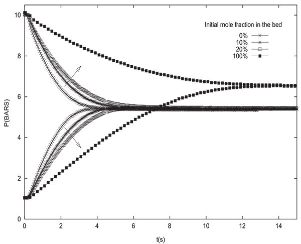
Fig. (16) gives a comparison between the values of the equilibrium pressure Peq obtained experimentally, numerically and analytically (from equation (14)). The values of PH and PL are 10 bars and 1 bar respectively. The initial methane molar fraction in the packed bed varies from 0 to 1. The experimental values are slightly underestimated by the numerical values and slightly overestimated by the analytical values. Indeed, the maximum difference does not exceed 0.1 bar when comparison is made with the experimental values. For the experiment with a column containing initially pure hydrogen (yCH4 =0), the experimental value of Peq obtained is 4.8 bars whereas the value given both by simulation and analytical solution is 4.88 bars. As previously mentioned, this slight difference is attributed to the fact of neglecting the volume of tubings connecting the packed bed and the tank. Indeed, the minimum value can not be lower than 4.88 bar obtained by the analytical solution (equation (22)) for a column containing only an inert gas or by simulation for the same case. The sole source of the discrepancies is to be attributed to the impact of the tubing volume. It is highly unlikely that the accuracy of the pressure measuring instrument is the cause of this deviation insofar as the value of the equilibrium pressure is obtained both by a manometer (pressure gauge) installed on the column (observable visually) and by a pressure transducer (electrical signal), the two values obtained are identical.
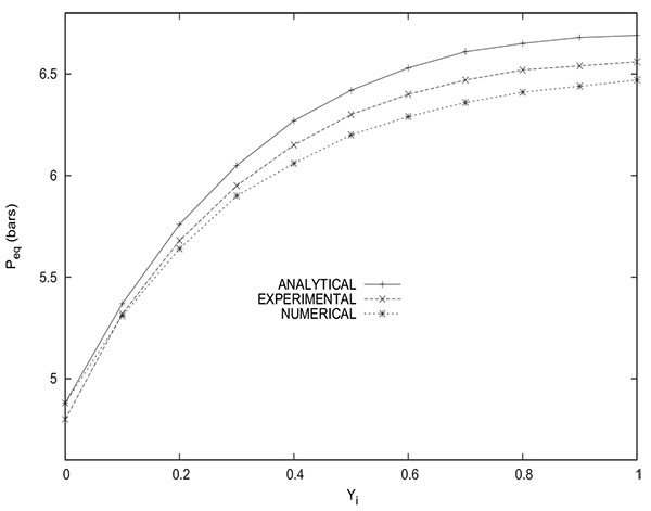
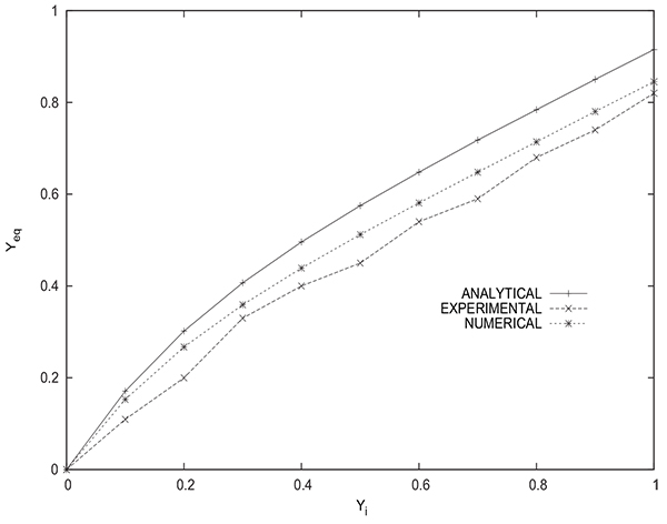
Fig. (17) shows a comparison between the values of the methane molar fraction Yeq in the tank at the end of the equalization step obtained experimentally, numerically and analytically (from equation (16)). It has to be mentioned that the experimental value of methane molar fraction in the tank is obtained by averaging the values for five samples of gas recovered from the tank after disconnecting it from the packed bed. The gas analysis is done by infrared absorption spectroscopy. The experimental values are close to the ones obtained by numerical simulation.The values given by the analytical solution are somewhat less precise, for example, the values obtained experimentally, numerically and analytically are 0.82, 0.84 and 0.91 respectively for the case of a bed initially saturated with pure methane (yCH4 =1). Hence, the numerical simulation of the equalization step is very satisfactory and allows to obtain reliable results either for the equilibrium pressure or mole fraction in the tank. The analytical solution gives acceptable results despite the simplifying assumptions considered, it permits to assess rapidly Peq and Yeq without the need to resort to a cubersome modeling.
One of parameters, among others, which contributes enormously to the optimization of the operation of pressure equalization is the tank volume Vtank . It should be borne in mind that the goals of this step are to maximize the pure product transfer from the column to the tank for increasing product recovery and to conserve mechanical energy.
In both cases, it is important that the adsorbable species molar fraction of the gas transferred to the tank at the end of pressure equalization is as low as possible. This would allow a better partial purge if the tank gas is used to partially purge a column just after the depressurization step, on one hand, and the preservation of the capacity of the adsorption column if the tank gas is used to pressurize a column at the end of a low pressure purge step on the other hand. It then becomes important to optimize the pressure equalization step so that the gas transferred from the column to the tank is minimally contaminated by the adsorbable species.
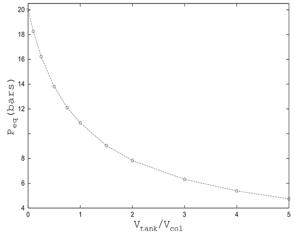
Fig. (18) shows the variation of Peq in function of the tank volume. The equilibrium pressure Peq decreases notably with Vtank . Thus, as an example, Peq =4.75 bars for Vtank =5.0Vcol and Peq =13.8 bars for Vtank =0.5 Vcol. It follows that increasing the volume of the tank presents the disadvantage of lowering enormously pressure. If the gas collected in the tank is intended for a column pressurization, one will have to choose the right volume of the tank so as to reach the desired pressure in the column to be pressurized at the end of the equalization step.
CONCLUSION
It is issential to pay a great attention when choosing models to simulate pressure swing processes. The pressure equalization step must be treated with special care since its impact on the assessment of the overall performance of the process is notable. If the equilibrium pressure is not accurately evaluated, this could lead inevitably to erroneous simulations in the case where the PSA cycle comprises a pressure equalization step. In fact, if rough approximations are considered, estimated Peq may differ from the real value leading to inaccurate simulation results. The analytical solution proposed herein for assessing the final pressure when connecting a bed and an empty tank could be considered acceptable despite the simplifying assumptions considered. Based on the comparisons presented, one can conclude that the agreement between the experimental and numerical results relative to the equilibrium pressure and the equilibrium mole fraction of the adsorbable species in the tank is very satisfactory, thus simulation results could be considered reliable and used safely so as to optimize PSA cycles. If the gas transferred to the tank is destined for subsequent column pressurization, the choice of the tank volume will depend on the value of the desired pressure to be reached in the column to be pressurized at the end of the equalization step.
NOMENCLATURE
| b | = parameter of Langmuir isotherm, P a−1 |
| C | = bulk phase concentration, mol/m3 |
| cp | = heat capacity, J /(molK) or J/(kgK) |
| cp | = mean intra-particle gas phase concentration, mol/m3 |
| Dax | = mass axial dispersion coefficient, m2/s |
| Dcol | = column diameter, m dp : Particle diameter, m |
| Dp | = pore diffusivity, m2/s |
| Ds | = surface diffusivity, m2/s |
| h | = heat transfer coefficient, W /(m2s) |
| H | = enthalpy, J /mol L: Bed length, m |
| Ng | = number of species in the gas mixture |
| P | = total pressure, P a |
| Q | = molar flow rate, mol/s |
| Qm | = parameter of Langmuir isotherm, mol/kg |
| q | = adsorbed phase concentration, mol/m3 or mol/kg |
| R | = gas constant or particle radius, J /(molK) or m |
| S | = cross section of the column, m2 |
| u | = interstitial velocity, m/s |
| U | = internal energy, J /mol |
| V | = volume, m3 |
| T | = temperature, K t: Time, s |
| Z | = compressibility factor of the gas mixture |
| z | = axial coordinate in the bed, m |
GREEK LETTERS
| ∆H | = heat of adsorption, J /mol |
| ϵ | = interparticle porosity |
| ϵp | = intraparticle porosity |
| ϵt | = total porosity |
| µ | = fluid viscosity, kg/(m s) |
| ρ | = fluid or bed density, kg/m3 |
| τ | = particle tortuosity factor |
SUPERSCRIPTS
| ∗ | = equilibrium |
| i | = refers to species i |
SUBSCRIPTS
| a | = refers to adsorbed phase |
| A | = refers to the adsorbable species |
| b | = refers to the bed |
| col | = refers to column |
| e | = refers to surroundings |
| eq | = refers to the equilibrium state |
| f eed | = at the bed entrance |
| g | = refers to gas phase |
| H | = refers to the high value |
| i | = refers to species i |
| I | = refers to the inert |
| L | = refers to the low value |
| out | = at the bed exit |
| p | = refers to adsorbent particle |
| s | = refers to solid phase |
| tank | = refers to tank |
| 0 | = initial condition |
CONSENT FOR PUBLICATION
Not applicable.
CONFLICT OF INTEREST
The authors declare no conflict of interest, financial or otherwise.
ACKNOWLEDGEMENTS
Declared none.