All published articles of this journal are available on ScienceDirect.
Review and Improvement of the Finite Moment Problem
Abstract
Background:
This paper reviews the Particle Size Distribution (PSD) problem in detail. Mathematically, the problem faced while recovering a function from a finite number of its geometric moments has been discussed with the help of the Spline Theory. Undoubtedly, the splines play a major role in the theory of interpolation and approximation in many fields of pure and applied sciences. B-Splines form a practical basis for the piecewise polynomials of the desired degree. A high degree of accuracy has been obtained in recovering a function within the first ten to fifteen geometric moments. The proposed approximation formula has been tested on several types of synthetic functions. This work highlights some advantages, such as the use of a practical basis for the approximating space, the exactness of computing the moments of these basis functions and the reduction of the size along with an appropriate transformation of the resulting linear system for stability.
Objective:
The aim is to recover a function from a finite number of its geometric moments.
Methods:
The main tool is the Spline Theory. Undoubtedly, the role of splines in the theory of interpolation and approximation in many fields of pure and applied sciences has been well- established. B-Splines form a practical basis for the piecewise polynomials of the desired degree.
Results:
A high degree of accuracy has been obtained in recovering a function within the first ten to fifteen geometric moments. The proposed approximation formula is tested on several types of synthetic functions.
Conclusion:
This work highlights some advantages, such as the use of a practical basis for the approximating space, the exactness of computing the moments of these basic functions and the reduction of the size along with the data transformation of the resulting linear system for stability.
1. INTRODUCTION
The Particle Size Distributions (PSD) is a key process used in several industrial operations such as chemical engineering, especially in dynamic multiphase flows. The size distribution of particles can be extremely important for several reasons. For example, this property may have an impact on the efficiency of processes like filtration. Indeed, small product sizes may result in a significant increase in processing time. Moreover, PSD generally represents a key result to assess the good quality of chemical process output. The evolution of the PSD depends on several parameters such as time, location, particle volume and chemical composition. Accessing experimentally the evolution of PSD through time is very complicated technically. Thus, most of PSD reconstruction techniques are based on numerical modeling. Simulation of such processes may require massive computational resources including a large amount of memory, the storage and access to the computed outputs during the simulation [1-6]
Several attempts of PSD reconstruction were proposed based on the orthogonal polynomials or continuous kernel functions. Some authors implemented the kernel density element method to approximate the PSD based on weighted kernel density functions [7]. The main limitation of this approach is the introduction of a quadrature error at moment closures. Other authors proposed to reconstruct the PSD using orthonormal functions such as Legendre polynomials without any assumptions on particle distribution [8]. Nevertheless, this approach may lead to negative cases of PSD as only a finite number of polynomials can be determined.
In addition, most of the applications implement a limited, finite number of moments for the reconstruction, highlighting possible inaccuracies. This constraint leads chemical engineering applications to be restricted only for very simple distribution shapes such as Gaussian or log-normal functions. In order to avoid such limitations, several authors proposed to model PSD using its few lower-order moments, while reducing computational cost [9-14]. Moments are defined as integrals of the PSD throughout particle ensemble. For example, the moment of order zero represents the total particle number and the first moment is the total particle mass. In the last decade, several research studies in chemical engineering focused on particle size distributions applications using moment-based techniques to determine distributions. Several authors have proposed different approaches to solve the reconstruction problem. A suitable PSD reconstruction technique should make sure that reconstructed PSD converges to the computed moments.
In addition to its importance to the field of chemical engineering applications, reconstructing a function from a finite number of its moments is an important step for many other problems encountered in Science and Technology such as electronic nuclear physics, image processing, and others. For example, in the field of tomography and image processing, we deal with the well-known application of reconstructing an image from its moments, or the reconstruction of the Radon Transforms from their moments [15-17].
Let ƒ be an unknown non-negative continuous function with compact support on the interval [a,b]. The geometric moments of an objective function ƒ are defined as:
 |
(1) |
Theoretically, we can determine ƒ from the given finite sequence Miƒ of all orders. However, encountered with an underdetermined problem, we tried to match up to the given, or allowed moments. Therefore, a numerical approach is presented to find a function that matches ƒ up to some order of moments. We can work with a shifted – scaled form of ƒ so that it is supported on the interval [0, 1] with 
Infact, the problem of determining ƒ from a given finite sequence Miƒ takes different forms due to the related physical and mathematical assumptions. Specifically, when moments of all orders are known, then ƒ can be recovered completely. Infact, the widely known Uniqueness Theorem of the moments [18] assures that the moments of all orders are uniquely determined by ƒ. Conversely, Miƒ of all orders uniquely determines ƒ. But, if only a finite number of these moments are given, then we may face the well-known inverse problem. Further, it is known that the support of the objective function ƒ categorizes the problem into different scenarios [14]. In the Hausdorff moment problem, the support of ƒ is a closed interval [a, b]. In the Stieltjes moment problem, the support of ƒ is on (0, +∞); and in the Hamburger moment problem, the support of ƒ is on (-∞, +∞).
Several reconstruction methods exist in the literature, mainly for the Hausdorff moment problem, but there is no unified method for the reconstructing problem. A great comparative study based on these various methods is discussed in a study [1]. A brief review of the known methods is as follows:
1.1. Parameter-Fitting Method
This method is limited to simple shapes. For example, a number of distributions have been listed below whose parameters are determined by the given low-order moments, (the first three moments), such as, the Gaussian-normal function, the Log-normal distribution, the Half-normal function, the Gamma function, and others [14].
1.2. Kernel Density Function-Based Method (KDF)
This approach was motivated by the above parameter-fitting method. It is based on a superposition of finite weighted kernel density functions for the Hausdorff moment problem and later was generalized to solve the Stieltjes moment problem [7]. KDF is a non-parametric method to estimate the probability density function for a random variable. This method is a positivity-preserving representation but needs a large number of the available moments to ensure accuracy. The objective function is approximated by a sum of N weighted kernel density functions as follows:
 |
(2) |
Where;
 are the KDFs, centered at xi, and is chosen as a Beta Kernel.
The bandwidth h of the kernel is a free parameter which exhibits influence on the resulting estimate and satisfies the coefficients cn.
 |
(3) |
The goal then is to determine the optimal coefficients cn. This problem is reformulated as a constrained optimization problem aiming to find the coefficients cn which minimizes the error between the set of initial moments and those estimated via the sum of Beta KDFs.
1.3. Maximum Entropy Method
The maximum entropy method requires less knowledge of the prior information or the number of moments, as compared to the Kernel density function-based method [9, 10]. It is based on the maximization of the Shannon entropy or the minimization of the relative entropy from information theory. The Shannon entropy is given by:
 |
(4) |
and the objective function is approximated by
 |
(5) |
The (N + 1) constraints are:
 |
(6) |
The (N + 1) Lagrange’s multipliers  are obtained by solving the nonlinear system of (N+1) equations:
 |
(7) |
1.4. Spline-Based Method
Spline approximation is a natural approach for the finite moment problem. For example, some authors tried the zero-order spline interoperation with a restriction on the recovered function. This approach may not be suitable for some applications, such as the PSD problem [13]. John et al. proposed the use of spline theory to the application of PSD problem with the advantage of no priori assumptions on ƒ [14]. In this case, the number of needed moments depends on the number of interpolation nodes. This approach divides the support of the [a,b] into N subintervals:
 |
On each subinterval  the target function is approximated by a cubic polynomial,
 |
(8) |
Thus, ƒ is piecewise-defined and is written as:
 |
(9) |
The unknown coefficients are the four coefficients of each spline, which is a total of 4N unknowns. A smoothness condition at the boundaries of the interval is assumed, which means that the function, its first and second derivatives, are null at the boundaries. This gives 2 × 3 equations. The continuity of the splines, their first and second derivatives at the nodes, provides 3(N − 1) equations. The remaining (N − 3) equations are supplemented from the moments by computing the moments of both sides of the equation (9):
 |
Hence, we can obtain N-3 equations from the equation
 |
(10) |
This leads to solve a 4N × 4N ill-conditioned linear system.
In this paper, a method to improve the existing spline approach has been proposed. Namely, the B-Splines expansions technique has been proposed to solve this problem. The key fact is that B-Splines of degree k form a basis for the linear space of piecewise polynomial functions of degree k. In fact, it is believed that our approach improves the approach presented above for two reasons:
a): The 4N × 4N ill-conditioned linear system needed for the above cubic splines approach is replaced by (N+3) × (N+3) system, and in general, we need N+k equations for B-splines of degree k.
b): The algorithm for this 4N × 4N system is sensitive to negative tolerance leading to different reconstructions for the same target function [1, 11].
The work is organized as follows the proposed methods are presented in Section 2.
Section 3 is concerned with experiments and discussion. Finally, in the last section, the conclusion is presented.
2. USING B-SPLINES FOR THE MOMENT PROBLEM
2.1. Background
A few definitions, concepts and facts obtained from the Approximation Theory are first reviewed. Mathematical literature provides a rich theory and tools for the classical interpolation and spline theory [19, 20]. Several options have been explored for approximating ƒ. In fact, using the B-spline functions serves and fits the physical, geometry, and settings of the current problem.
Starting with a partition of the interval [a,b], as given by the following equation
 |
(11) |
that divides this interval into N subintervals.
Let S(k,∆N) be the linear space of piecewise polynomial functions of degree k with knots ∆N.
A function sϵS(k,∆N) if
(i) On each subinterval  coincides with a polynomial of degree ≤ k
(ii) s ϵ Ck-1[a,b], so s has k-1 continuous derivatives.
Further, the dimension of the space S(k,∆N) is N + k.
One way of introducing the B-splines is to address the question of choosing a basis for S(k,∆N) so that each member of this basis is identically zero over a large part of the range [a,b]. The family of B- splines of degree k provides such a basis. Considering the above partition ∆Neach B-spline,  is a polynomial of degree k. The subscript p denotes that the support of
  is the interval
  , so that
  is zero outside this interval. A known recursion formula of the B-splines of degree k at the knots
  is given by Cox-de Boor Recursion Formula [22]:
 |
(12) |
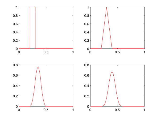
Fig. (1) shows B-splines of degrees 0,1,2, and 3 with a uniform partition.
This section has been concluded with the following key points [19], showing that B-splines can be used as a basis for the space S(k,∆N).
Theorem 1:
Consider the extended partition 
 .
.
The set  forms a basis for S(k,∆N).
Thus, if sϵ(k,∆N), then s(x) =  for some coefficients.
 |
(13) |
2.2. The Theory
Returning to our current problem, Let ƒ be an unknown nonnegative function with compact support on the interval [a,b]. A spline approximation s(x) for ƒ from S(k,∆N) is required such that
 |
(14) |
In order to use the given moments of ƒ, we make the following two observations:
First, if  is normalized so that
  then equations (2) and (6) will be formed:
 |
(15) |
Second, the j-th moment of the normalized  , can be expressed as Carlson's Dirichlet Average [21] which in turn can be solved via a contour integral and an iterative sum [22] as:
 |
(16) |
and D0 = 1. Here Γ is the Gamma function,  , is the vector of knots in the support of
  , m is the vector of their multiplicities and m is the sum of the components of m.
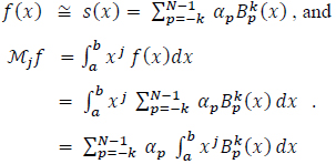
Consider the moments of both sides of (14):
 |
(17) |
The linear system representation of (17) is written as:
 |
(18) |
Where A is (N + k) X (N + k) matrix of B-splines moments on the interval [a, b], α is the vector of the N + k unknown coefficients and Mƒ is the vector of the known - k, 0, ...,N - 1 moments of ƒ.
Notice that we need to pay attention when using Equation (16) to fill the matrix A ; namely, adjustments regarding those splines whose supports are partially beyond the interval [a, b]. This endpoint concern will be discussed later. Equation (18) can be ill-conditioned for a large size computation. More details on this system are presented in the discussion section.
3. DISCUSSION AND EXAMPLES
Following the discussion of Section 2, the B-spline approximation of the function ƒ on the interval [0,1] ƒ(x)  s(x) as in Equation (14), with degree k = 3, will now be considered. For the cubic B-splines, we use the partition
 |
With this particular value of the degree (k=3); Equation (14) becomes,
 |
(19) |
We proceed Equation (17) by computing the moments of Equation (19):
 |
We explicitly display the first and last three terms of this summation:
 |
(20) |
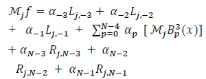
For a more compact notation, we write the left three terms as
 |
And the right three terms as:
 |
Then, Equation (20) with the values j = 0,1, ... , N + 2 gives the (N + 3) X (N + 3) system:
 |
(21) |
System (18), built from (21), can be ill-conditioned for a large size computation. We treat this behavior by the following transformation of data: Let A = QR be the QR-factorization, which is a decomposition of the matrix A where R is an upper triangular matrix and Q is an orthogonal matrix i.e. QQT = I where T denotes the transpose and I is the identity matrix. Then, one can show that the system (18) is equivalent to
 |
(22) |
that can be solved by back substitution.
We also need measures of error. Define
 |
(23) |
This measures the closeness s of ƒ
Along with this discussion, we consider some examples. All the experiments are conducted using MATLAB.
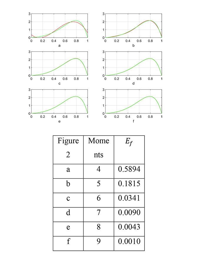
Example 1. In Fig. (2), we show the function: ƒ(x) = sin(πx)e4x normalized on [0,1] with the moments: N = 4,5,6,7,8 and 9, along with the corresponding error (23).
Another example of our tests:
Example 2. We consider the function:
ƒ(x) = exp [-80(x - 0.3)2] + exp [-80(x - 0.6)2] +
  normalized on [0,1], with moments with moments N = 10,11,12,13,14, and 15. Results are shown in Fig. (3)
We now address a number of concerns regarding our approach; we summarize these concerns in the following three remarks:
Remark 1: On approximation with polynomials
The Weierstrass approximation theorem [23], states that for every continuous function ƒ(x) defined on an interval [a,b], there exists a set of Polynomials pi(x), i ≤ N that approximates ƒ(x) with uniform convergence over [a,b] as N→∞ . However, this theorem does not provide a general method of finding such a set of polynomials. A set of polynomials may even diverge as N increases. This typically occurs in an oscillating pattern that magnifies near the ends of the interpolation points. This is known as Runge's phenomenon [24]. In fact, oscillation at the edges of an interval occurs when polynomials of a high degree over a set of equispaced interpolation points are used. The phenomenon is similar to the Gibbs phenomenon in Fourier series approximations [25]. According to Runge's phenomenon, the magnitude of the n-th order derivatives of this function grows quickly for a large degree and the equidistance between points, which leads to a larger Lebesgue constant for large N.
In the classical interpolation practice, we mitigate this issue using different approaches, such as change of interpolation points, use constrained minimization, use of piecewise polynomials, Least-squares fitting, and others.
Although our research problem here is not a classical interpolation, since interpolations require the knowledge of a sample of ƒ(x) on [a,b], we indeed adapted the use of piecewise polynomials, the B-splines.
Remark 2: Convergence Property of Spline Approximation
When we require a B-Spline interpolation s from S(k,∆N) to a function ƒ on the interval [a,b], we need to have a bound on the least maximum error:
 |
(24) |
It is known that [19],
 |
(25) |
where ω is the modulus of continuity of  , and k is t QR the spline degree.
It follows that any continuous function can be approximated to arbitrarily high accuracy by a spline function s(x) =  , provided that the spacing between the knots is sufficiently small.
However, our study, as said, is not an interpolation problem and the use of a large N brings other
limitations, as explained in the next remark.
Remark 3: Limitations
Although our approach never needs a large N, it is important for the completeness of this discussion to address this point. Consider the system Aα = Mƒ in Equation (18), given in a more explicit form by Equation (21):
 |
Each j generates one equation of this system, j = 0,1, ... , N + 2; and the entries of the coefficient matrix A are decreasing as j increases. For example, the coefficient of the first unknown α-3 is
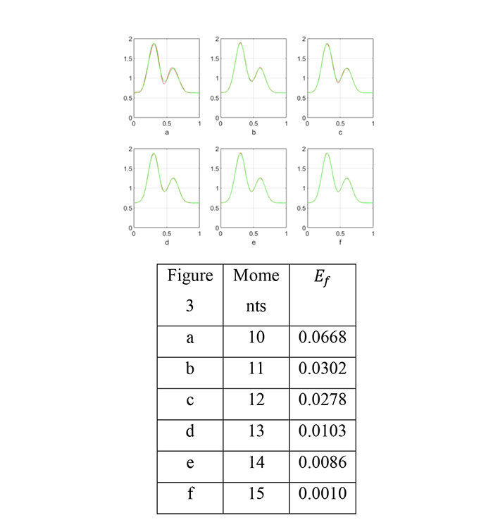
 exp [-80(x - 0.6)2] +
  normalized on [0,1] and s(x) from (19) along with Eƒ for different moments.
 |
This may explain why a large N makes the matrix A singular. The QR factorization can reduce the instability of this system. However, for a large N, this approach would not work.
CONCLUSION
Recovering a function from a finite number of its geometric moments is a known ill-posed problem. The literature-based on this topic has been reviewed, and a significant improvement for the spline approach has been proposed to solve this problem. It has been observed that approximating the target function from its moment in terms of a piecewise polynomial is one of the efficient, and stable approaches, in particular when the basis of such a space of functions is a family of B-Splines. Results show good accuracy in recovering different types of synthetic functions. In fact, this work brings some advantages as compared to the existing approaches, such as the use of a practical basis for the approximating space, the exactness of computing the moments of these basis functions and the reduction of the size along with the QR transformation of the resulting linear system for stability.
CONSENT FOR PUBLICATION
Not applicable.
FUNDING
None.
CONFLICT OF INTEREST
The author declares no conflict of interest, financial or otherwise.
ACKNOWLEDGEMENTS
Declared none.


