All published articles of this journal are available on ScienceDirect.

On Orthogonal Polynomials and Finite Moment Problem
Abstract
Background:
This paper is an improvement of a previous work on the problem recovering a function or probability density function from a finite number of its geometric moments, [1]. The previous worked solved the problem with the help of the B-Spline theory which is a great approach as long as the resulting linear system is not very large. In this work, two solution algorithms based on the approximate representation of the target probability distribution function via an orthogonal expansion are provided. One primary application of this theory is the reconstruction of the Particle Size Distribution (PSD), occurring in chemical engineering applications. Another application of this theory is the reconstruction of the Radon transform of an image at an unknown angle using the moments of the transform at known angles which leads to the reconstruction of the image form limited data.
Objective:
The aim is to recover a probability density function from a finite number of its geometric moments.
Methods:
The tool is the orthogonal expansion approach. The Shifted-Legendre Polynomials and the Chebyshev Polynomials as bases for the orthogonal expansion are used in this study.
Results:
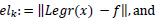
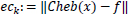
A high degree of accuracy has been obtained in recovering a function without facing a possible ill-conditioned linear system, which is the case with many typical approaches of solving the problem. In fact, for a normalized template function f on the interval [0, 1], and a reconstructed function
 ; the reconstruction accuracy is measured in two domains. One is the moment domain, in which the error (difference between the moments of f and the moments of
) is zero. The other measure is the standard difference in the norm -space ||f-
|| which can be ≈ 10-6 or less.
; the reconstruction accuracy is measured in two domains. One is the moment domain, in which the error (difference between the moments of f and the moments of
) is zero. The other measure is the standard difference in the norm -space ||f-
|| which can be ≈ 10-6 or less.
Conclusion:
This paper discusses the problem of recovering a function from a finite number of its geometric moments for the PSD application. Linear transformations were used, as needed, so that the function is supported on the unit interval [0, 1], or on [0, α] for some choice of α. This transformation forces the sequence of moments to vanish. Then, an orthogonal expansion of the Scaled Shifted Legendre Polynomials, as well as the Chebyshev Polynomials, are developed. The result shows good accuracy in recovering different types of synthetic functions. It is believed that up to fifteen moments, this approach is safe and reliable.
1. INTRODUCTION
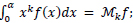
Consider an unknown nonnegative function f with compact support on the interval (
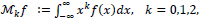 |
(1) |
In fact, the problem of determining f from a given finite sequence Mkf takes different forms due to the related physical and mathematical assumptions. Specifically, if Mfk is known for all orders, then f can be recovered completely, but if only a finite number of these moments are given, then we have the well-known inverse ill –conditioned problem. Furthermore, it is known that the support of the objective function f categorizes the problem into different scenarios [1-4]. The Hausdorff moment problem, where the support of f is a closed interval (a, b), the Stieltjes moment problem, where the support of f on (0, +∞), and the Hamburger moment problem, where f is supported on (−∞, +∞).
Reconstructing a function from a finite number of its moments is an essential tool for many problems in science and technology. Among many applications that involve the moment problems, three major fields are described. Namely, chemical engineering applications, tomography, and image processing. The most known existing methods of solving the moment problem are reviewed in [1]. A general review of these applications is now given.
In the field of chemical engineering, the Particle Size Distribution (PSD) is a crucial process that results in several industrial operations in chemical engineering, especially in dynamic multiphase flows. The size distribution of particles can be essential for several applications. For example, this property may have an impact on the efficiency of processes like filtration, as a small product size may result in a significant increase in processing time. Moreover, PSD generally represents a pivotal result to assess the excellent quality of chemical process output. Methods to retrieve PSD can be divided into three main categories [1-4]. The first approach is based on analytical inversion techniques. In the second approach, PSD is recovered using discrete linear equations sets implemented in the independent model algorithm. The third approach consists of reconstructing PSD from known moments. In the last decade, several research studies in chemical engineering focused on PSD applications using moment-based techniques to determine distributions [4-10]. Moreover, most of the applications implement a limited, finite number of moments for the reconstruction introducing possible inaccuracies. This moment constraint makes chemical engineering applications restricted only to elementary distribution shapes such as Gaussian or lognormal functions.
Moment-based approach for several types of image processing and tomography problems attracted the attention of many researchers, for instance [11-20]. For example, in image processing, we compute the image moments from the given projections for the purpose of shape classification or object position and orientation, recovering a general linear transformation of images, segmentation, texture analysis [12-16], and others. In the field of tomography, including digital rock physics, we deal with the well-known application of reconstructing an image from its moments or the reconstruction of the Radon Transforms from their moments [17-21]. Specifically, we use the connection between the projection moments and the image moments, and the connections among the projection moments from different views. Using these known relations [13-17], we obtain all possible image moments from the given projections. The image can then be recovered.
As said, a full review of the most known existing methods of solving the moment problem is reviewed [1].
This work considers the Hausdorff moment problem and proposes the use of orthogonal polynomial expansion techniques to solve this problem. Without loss of generality,
This work is organized as follows: In the next section, our proposed method is presented. Section 3 is concerned with experiments and discussion. Finally, the conclusion can be found in the last section.
2. MATERIALS AND METHODS
Our tool is the orthogonal expansion. Mathematics Literature provides a rich theory and tools for the classical orthogonal expansion of functions [22-29]. The choice of several options of orthogonal bases that serve and fit the physical, geometry, and settings of our current problem is explored. Undoubtedly, the role of the Fourier series, the Legendre’s and Chebyshev polynomials in many fields of pure and applied sciences are well-established. An orthogonal expansion that allows us to represent the expansion's coefficients in terms of the moments rather than the function itself since it is not known, is required. It is found, for example, that the Fourier series is not relevant to this problem. Expressing the Fourier series coefficients in terms of moments is possible, but the numerical implementation immediately would suffer the overflow issues. On the other hand, the Legendre series and Chebyshev series proved very well stable solutions using a few moments of the target function.
2.1. Using Legendre Polynomials
The Legendre polynomials ϕm(x) form a complete orthogonal system over the interval [-1,1]:
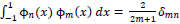 |
(2) |
where δmn denotes the Kronecker delta.
Since we require an approximation on the interval [ 0,1], we first use the mapping (transformation)
 |
(3) |
that moves the interval [0,
 |
(4) |
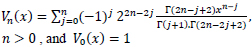
We have a handy explicit formula for
 |
(5) |
The Legendre series for
 |
(6) |
By orthogonality of
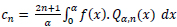 |
(7) |
Using (5), we write (7) as:
 |
 |
(8) |
But
 so (8) is written as:
 |
(9) |
Using (9), equation (6) is written as:
 |
(10) |
If we consider the N-partial sum of (10), we obtain:
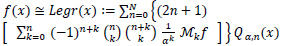 |
(11) |
Thus, the approximating function
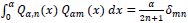
2.2. Using Chebyshev Polynomials
The Shifted Chebyshev Polynomial of the second kind [25], say
 |
(12) |
with the weight function
 |
(13) |
We can express our objective function in the following manner:
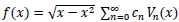 |
(14) |
Using (12), we solve for the coefficients,
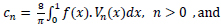 |
(15) |
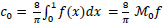 |
(16) |
Using (13), we write (15) as
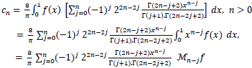 |
(17) |
Thus, (14) is written as
 |
(18) |
Finally, we consider the partial sum of (18) to obtain:
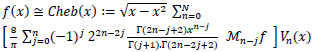 |
(19) |
Examples and discussion of these results are given in the next section.
3. RESULTS AND DISCUSSION
Now, the following remarks concerning our method are addressed. First, in (3.1), our theory using synthetic functions is tested and validated using MATLAB. In doing so, moments of order up to fifteen or less are employed, and a reliable approximation using either one of the two families of polynomials of this study is shown. Second, in (3.2), the behavior of a series of polynomials with a large number of terms and other properties is considered. This work is not a classical interpolation since interpolation requires a sample of the objective function. In the classical theory of interpolation, the Chebyshev series is believed to be a better approximation if the interpolation nodes are chosen to be the Chebyshev nodes. In the context of this work, the two series (11) and (19) are not comparable in terms of accuracy, given that we want to rely on a few terms of these series. However, they exhibit different behaviors in regard to errors. Overall, thanks to the restriction of using only a few moments, we will not need many terms. It is believed that up to fifteen moments, this approach is safe and reliable.
3.1. Demonstration
In testing our formulas (11) and (19), the support of the testing functions will be the interval (0,
 |
(20) |
 |
(21) |
As a first example, we consider the function:
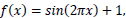 |
(22) |
| Figure 1 | Moment N |
|
|---|---|---|
| a | 2 | 0.9584 |
| b | 4 | 0.2084 |
| c | 6 | 0.0662 |
| d | 8 | 0.0092 |
| e | 10 | 0.0004 |
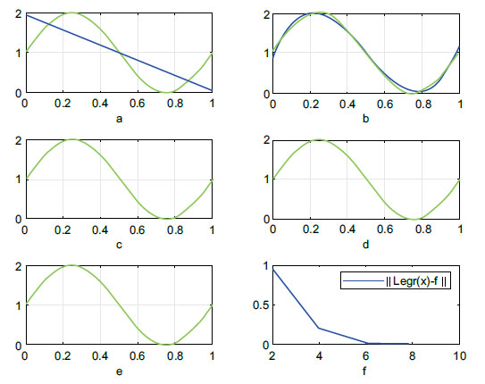
different moments:
In the second example, consider the function:
 |
(23) |
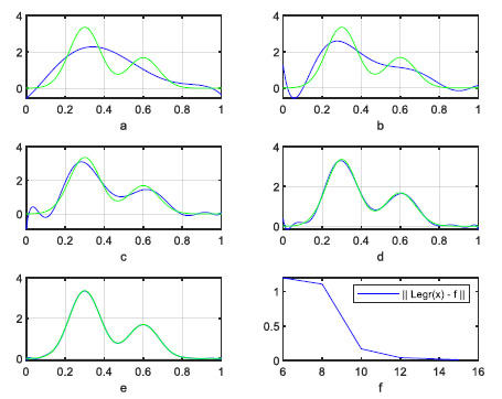
| Figure 2 | Moment N |
|
|---|---|---|
| a | 6 | 1.1954 |
| b | 8 | 1.1054 |
| c | 10 | 0.1682 |
| d | 12 | 0.0396 |
| e | 15 | 0.0037 |
The assumption that f(0) = f(1) = 0 is natural in some applications. For example, in image processing and tomography, we can assume that the image is supported in the interior of the unit circle. Similarly, we consider the value of PSD out of the support (0, 1) to be small enough and can be set as zero. For the rest of our experiments and discussion, we will be under this assumption.
recovered using (19) with different moments:
Working with both families of polynomials, we test
Results are shown in Table 3 and Fig. (3). Both are approximated very well using either (11) or (19) within the first twelve moments.
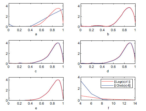
| Figure 4 | Moment N |
||
|---|---|---|---|
| a | 3 | 0.0389 | 0.0067 |
| b | 5 | 0.0220 | 0.0060 |
| c | 7 | 0.0046 | 0.0034 |
| d | 10 | 0.0001 | 0.0085 |
| e | 12 | 0.0000 | 0.0015 |
different moments:
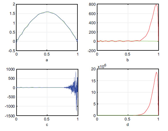
3.2. The Case of Large N
Although our approach never needs a large N, the completeness of this discussion needs to address several concerns regarding the approximation by polynomials. The Weierstrass approximation theorem [25] states that for every continuous function
In the classical interpolation practice, this issue using different approaches is mitigated, such as change of interpolation points, using the S-Runge algorithm without resampling, use of constrained minimization, use of piecewise polynomials, Least-squares fitting, and others. Perhaps, the most common of these is the standard Chebyshev points. Although our work here is not a classical interpolation since interpolations require the knowledge of a sample of
For visual display, we repeat the test of the function
CONCLUSION
This paper discusses the problem of recovering a function from a finite number of its geometric moments for the PSD application. Linear transformations were used, as needed so that the function is supported on the unit interval
[0, 1], or on [0,
LIST OF ABBREVIATIONS
| PSD | = Particle Size Distribution |
| f | = Function |
CONSENT FOR PUBLICATION
Not applicable.
AVAILABILITY OF DATA AND MATERIALS
The data supporting the findings of the article is available within the article.
FUNDING
None.
CONFLICT OF INTEREST
The authors declare no conflict of interest, financial or otherwise.
ACKNOWLEDGEMENTS
Declared none.